49 Wave spectra

Mathematically, an arbitrary time-series of length T can be very closely approximated by the sum of a (possibly large, theoretically infinite) number, N, of sinusoidal functions, called wave components.

This representation is called a Fourier series or Fourier decomposition, For some very nice examples of how some common functions are represented, see Dan Russell’s webpage Fourier Series and Waves. (On his webpage, the height of the red bars shows the amplitude of sinusoidal components of increasingly higher frequency that are added together to make the function of time on the left.)

Fourier decomposition leads to a representation of time-series data in the form of a spectrum, where the frequency, , appears on the x-axis and the squared amplitude (often divided by the frequency) appears on the y-axis. Logarthmic scales are commonly used. Because the amplitude of the displacement is related to the wave energy, the spectrum shows how the energy of a wave field is distributed among its wave components. An example ocean wave spectrum is shown below.

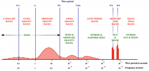
Atmospheric forcing (for example a storm) creates a disturbance of the ocean surface at a given point in time and space, that could be represented mathematically by a Fourier series. The individual wave components propagate across the ocean, and can travel thousands of kilometers before breaking on distant shores. The shape of the sea surface at a given time and place is composed of the interference patterns of waves created by different wind forcing events traveling in different directions.