14 The Turbulent Diffusive Flux

We will not go into the details of the physics of turbulence in this course.  At this point, our main concern is that turbulence is associated with a much more efficient “diffusion” of properties in a fluid compared to molecular diffusion.

Both larger scale flow and the turbulence are advective processes. Recall that the advective flux is the property concentration (C) times the velocity.  Here we are going to just look at the flux in the x-direction.

In the last expression, we have broken both the concentration and the velocity up into two components: a time-mean component indicated by an overbar, and a component that can fluctuate in time (but that has zero mean itself).  Realistically, this overbar might indicate averaging for about a half hour – that’s about the minimum amount of time it takes to get a good picture of the statistics of the turbulence in the ocean. Thus the overbar is not a truly a long-term mean – it represents the larger scale flow field that is changing more slowly than a timescale of an hour or so.

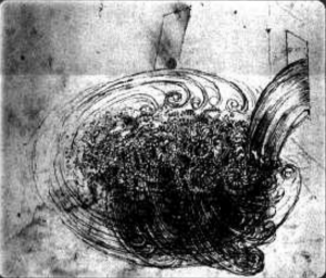
Note: This separation of time- and space-scales of motion is called the Reynolds Decomposition, and echoes an observation of Leonardo da Vinci:

We will multiply out the last expression

Now we will take the time average of each of these terms

(1) For the first term, the time average of the product of the two time averages is redundant since these are just constants in time.  Physically this represents the advective flux of the property by the larger scale flow field.

(2) The second term is identically zero.  The time-average concentration is just a number and the fluctuating part has zero time average, so their product is zero.

(3) Similarly, the third term is identically zero.

(4) The fourth term represents a time averaged correlation between velocity and property fluctuations.  Physically, this term represents the turbulent transport of the property.

Simplifying:

If we have an instrument capable of resolving the turbulent fluctuations we can measure the turbulent transport, directly.  But these measurements are typically expensive.  So we try to model the turbulent transport in terms of things we already know about the larger scale flow and property fields.

One simple and widely used model of this process is to model turbulent transport using Fick’s Law of diffusion, but with a diffusivity that is much (several orders of magnitude in the ocean) larger than the molecular diffusivity.

We usually drop the overbars from the time-mean quantities.

Here is an example (artificial) time series of vertical velocity (w, top right) and temperature (T, top left) with zero mean flow, but an underlying upward turbulent transport of heat. The bottom left panel shows the individual  pair at the instant indicated by the red dot in the time series on the top row.  The value of the time-averaged turbulent temperature transport (determined by a least-squares line fit to the scatter plot in the lower left corner) is:

To get turbulent heat transport, we would multiply by fluid density and heat capacity.

Mathematically, positive heat flux is associated with a statistical correlation between velocity and temperature anomalies. You can see this graphically from the quadrants that the individual points appear in – both the first quadrant ( and ) and the third quadrant ( and ) will result in a positive product of the two quantities.