
33 Geostrophic balance
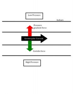
If the Rossby number is low, then rotation is important. The steady-state force balance between the Coriolis force and the pressure gradient force is called geostrophic balance and is the approximate state of most large-scale flows in the ocean and atmosphere. For example, the y-component momentum equation in geostrophic balance (see figure at left) would be written:
![\[ 0 = -fu-\frac{1}{\rho_0}\frac{\partial P}{\partial y} \]](https://uw.pressbooks.pub/app/uploads/quicklatex/quicklatex.com-b81bce7ba4914679a7b98c25e47deb4d_l3.png "Rendered by QuickLaTeX.com")
Since the current vector is perpendicular to the Coriolis force, it is also perpendicular to the pressure gradient. Flow is thus along lines of constant pressure, called isobars, rather than down the pressure gradient as we would intuit from the smaller scales of our everyday experience.
Key Takeaways
If the pressure field is known, then the geostrophic velocity components can be directly calculated as:
![\[ u =- \frac{1}{f \rho_0 }\frac{\partial P}{\partial y} \]](https://uw.pressbooks.pub/app/uploads/quicklatex/quicklatex.com-bfbe7c401b928b398a1d25f77da0e68c_l3.png "Rendered by QuickLaTeX.com")
![\[ v = \frac{1}{f \rho_0 }\frac{\partial P}{\partial x} \]](https://uw.pressbooks.pub/app/uploads/quicklatex/quicklatex.com-39a3f4e5d2a3e3654675ac1fb7c7dff5_l3.png "Rendered by QuickLaTeX.com")
However, unlike the atmosphere, the pressure field in the ocean is quite difficult to measure. Near the surface of the ocean, the shallow pressure field can be measured by satellite altimeters. The shallow pressure is related hydrostatically,  , to the elevation of the sea surface,
  relative to its equilibrium geopotential, z = 0.
This technology alone is particularly useful for detecting how currents change in time because estimates of the time-mean state require knowledge of the gravity field with a high degree of accuracy.
Key Takeaways
The near-surface geostrophic flow can be calculated from sea surface height as:
![\[ u_{surface} =- \frac{g}{f }\frac{\partial \eta}{\partial y} \]](https://uw.pressbooks.pub/app/uploads/quicklatex/quicklatex.com-9fa6a4582bccae46f29aee77bdc07c7b_l3.png "Rendered by QuickLaTeX.com")
![\[ v_{surface} = \frac{g}{f}\frac{\partial \eta}{\partial x} \]](https://uw.pressbooks.pub/app/uploads/quicklatex/quicklatex.com-5ce95a56bfde5824f6d0444a32358177_l3.png "Rendered by QuickLaTeX.com")
In the interior ocean, we cannot measure horizontal pressure gradients directly, but we can use CTD data to measure dynamic height, related to the difference in the pressure gradient between two levels in the vertical.
Key Takeaways
Differences in geostrophic velocity in the vertical (between two pressure levels) can be found from measured horizontal dynamic height gradients:
![\[ u(P)-u(P_{REF}) =- \frac{1}{f }\frac{\partial D}{\partial y} \]](https://uw.pressbooks.pub/app/uploads/quicklatex/quicklatex.com-ee046f001093a75da392e5d1feec8289_l3.png "Rendered by QuickLaTeX.com")
![\[ v(P)-v(P_{REF}) = \frac{1}{f}\frac{\partial D}{\partial x} \]](https://uw.pressbooks.pub/app/uploads/quicklatex/quicklatex.com-3b0d93735da63f9dd90a37a974fb8680_l3.png "Rendered by QuickLaTeX.com")
where in this case
![\[ D=-\int_{P_{REF}}^{P}\frac{1}{\rho}dP \]](https://uw.pressbooks.pub/app/uploads/quicklatex/quicklatex.com-44ecada0a7892a429d8eba5288749bf2_l3.png "Rendered by QuickLaTeX.com")
A common assumption about the reference level ( ) velocity is that it is zero at some deep level (i.e., that it is much smaller than the velocity of interest, typically a stronger, shallower flow). Alternately, the geostrophic velocity can be measured directly at the reference level.
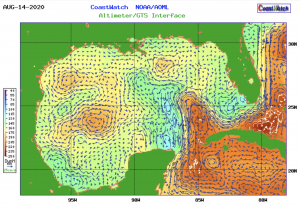
This map shows geostrophic currents on a particular day. First, an estimate of the time-mean geostrophic circulation is made that applies near the surface of the ocean, using an optimal fit to combined data from satellite altimeters, density profiles, and drifting buoys. This time-mean field is then added to the time-variable field (that can accurately be determined from altimeter data) to produce daily operational maps of ocean currents.
Media Attributions
- Geostrophic_current © Ncswart on Wikimedia Commons is licensed under a CC BY-SA (Attribution ShareAlike) license
- GulfofMexicoGeostrophicCurrents © NOAA Atlantic Oceanographic and Meteorological Laboratory is licensed under a Public Domain license
