
37 Sverdrup transport
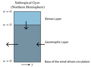
Ekman pumping will create a vertical divergence or convergence in the geostrophic layer below. Consider a northern hemisphere subtropical gyre with a uniform x-component of the pressure gradient that gives rise to a y-component of geostrophic flow,
![\[ v=\frac{1}{\rho_0 f}\frac{\partial P}{\partial x}. \]](https://uw.pressbooks.pub/app/uploads/quicklatex/quicklatex.com-3c857615004d484f415a883fac25e1e6_l3.png "Rendered by QuickLaTeX.com")
Since the magnitude of the geostrophic velocity is inversely proportional to the Coriolis parameter, the speed must be lower at higher latitude. If the current is southward, as shown in the figure, there is horizontal divergence. To conserve mass, this would need to be compensated by vertical convergence, i.e., downwelling from the Ekman layer. In reality, of course there are two horizontal components of geostrophic flow, but this intuitive reasoning still applies.
Mathematically, we can derive the horizontal divergence of the geostrophic velocity as
![\[ \frac{\partial u}{\partial x}+\frac{\partial v}{\partial y} = \frac{1}{\rho_0}\frac{\partial}{\partial x}\left(-\frac{1}{f}\frac{\partial P}{\partial y}\right)+\frac{1}{\rho_0}\frac{\partial}{\partial y}\left(\frac{1}{f}\frac{\partial P}{\partial x}\right) \]](https://uw.pressbooks.pub/app/uploads/quicklatex/quicklatex.com-01019fc0ec4be9b3770f728a569b0829_l3.png "Rendered by QuickLaTeX.com")
The Coriolis parameter only depends on y, so we will expand the last term via chain rule to
![\[ \frac{\partial}{\partial y}\left(\frac{1}{f}\frac{\partial P}{\partial x}\right) =\frac{1}{f} \frac{\partial}{\partial y}\frac{\partial P}{\partial x} - \frac{\partial f / \partial y}{f^2}\frac{\partial P}{\partial x} \]](https://uw.pressbooks.pub/app/uploads/quicklatex/quicklatex.com-a2e567f70a81408174a44bb4ce1f5051_l3.png "Rendered by QuickLaTeX.com")
Now we recognize that the order of the partial derivatives can be reversed, such that the first term on the right cancels with  . We will use the symbol
  for the y-derivative of the Coriolis parameter,
  , and substitute in the geostrophic velocity,
  , to get
![\[ \frac{\partial u}{\partial x}+\frac{\partial v}{\partial y} = - \frac{\beta}{f}v \]](https://uw.pressbooks.pub/app/uploads/quicklatex/quicklatex.com-8ce923ab1694f1e0be6fe7b416941986_l3.png "Rendered by QuickLaTeX.com")
If we assume the velocity is zero at some depth in the fluid that indicates the base of the wind-driven circulation, z = –D, then the vertical divergence due to Ekman pumping is
![\[ \frac{\partial w}{\partial z}=\frac{w_{Ekman}-0}{D}. \]](https://uw.pressbooks.pub/app/uploads/quicklatex/quicklatex.com-b324dcfe6db3b57036be82b69a9fde62_l3.png "Rendered by QuickLaTeX.com")
In this simple two-layer representation, the lower layer should have a thickness of  , but we can assume that the Ekman layer is much thinner than the depth of the wind-driven flow
  , and so only
  appears in the denominator. Since the sum of the divergence in the vertical and horizontal must be zero, we get
![\[ \frac{\partial u}{\partial x}+\frac{\partial v}{\partial y}=-\frac{\partial w}{\partial z} \]](https://uw.pressbooks.pub/app/uploads/quicklatex/quicklatex.com-2ddbdddfec57ea8a269bbc6d5d312ed0_l3.png "Rendered by QuickLaTeX.com")
or,
![\[ \frac{\beta}{f}v = \frac{w_{Ekman}}{D} \]](https://uw.pressbooks.pub/app/uploads/quicklatex/quicklatex.com-3de80e6c91047bf5d1b17581a8273011_l3.png "Rendered by QuickLaTeX.com")
Since we can relate the Ekman pumping velocity to the wind stress curl, and recognize the product of geostrophic velocity and depth as the transport per unit width  , we can arrive at a final expression for the geostrophic transport below.
Key Takeaways
Sverdrup balance is a theory predicting the geostrophic transport in the ocean from the wind-stress field (in m2 s-1, i.e., per unit width )
![\[ \frac{\beta}{f}vD = \frac{\beta}{f}Transport_{Geostrophic}^y = \frac{1}{\rho_0} \nabla \times \left( \frac{\underline{\tau}_{WIND}}{f} \right) \]](https://uw.pressbooks.pub/app/uploads/quicklatex/quicklatex.com-cf5fac67b45e0e8ac05aeec2fc759d85_l3.png "Rendered by QuickLaTeX.com")
Where there is a positive wind stress curl, Sverdrup transport will be toward the pole. Similarly, where there is a negative wind stress curl, Sverdrup transport will be toward the equator.
Media Attributions
- SverdrupBalance © Susan Hautala is licensed under a CC BY-NC-SA (Attribution NonCommercial ShareAlike) license
