Estimating Derivatives from Data

Susan Hautala

6 Estimating Derivatives from Data

If we want to use these ideas in real world problems, we need to be able to estimate partial derivatives using data.

Here is some pretend data – for concreteness’ sake let’s say that the y-axis is pressure (perhaps from from sea-surface height measured by a satellite altimeter). For example, it might be the pressure as a function of distance to the east (x) holding depth (the z-coordinate) and latitude (the y-coordinate) fixed.

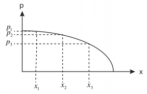
p(x) at z = -50 m and y = 24°N

We want to use our measurements of pressure at discrete values of longitude (x_i) to estimate the first- and second- partial derivatives of pressure with x. For example, we could use the first partial derivative to estimate the pressure gradient at, say, x₂. As another example, when we work problems involving diffusion, we might need to estimate the second partial derivatives.

Estimating the first partial derivative

In the example above, the first partial derivative at x₂ is approximated by the change in p divided by the change in x (i.e., the “rise” over the “run” to get the approximate slope of the tangent line at x₂.

Key Takeaways

We can estimate the first partial derivative using a finite difference approximation to the partial derivative of pressure with respect to x:

$\frac{\partial p}{\partial x}\bigg|_{x_2}\approx\frac{\Delta p}{\Delta x}=\frac{p(x_3)-p(x_1)}{x_3-x_1}$

Why did we use points 1 and 3? If we used either points 1 and 2, then the resulting tangent line would have a slope that is more appropriate to a point that lies between points 1 and 2. Since we want the tangent line slope at x₂, we choose to take a difference using points that are centered on point 2. Not surprisingly, this is called using a centered difference approximation. Had we used points 1 and 2 to calculate our $\Delta$ values, then we would have used a backward difference approximation (because we used information for values lower than, or behind, x₂). Had we used points 2 and 3, we would have used a forward difference approximation.

Estimating the second partial derivative

The second derivative (or the derivative of the first derivative) gives you the rate of change of the slope of the tangent line with x. As an example, if the second derivative is zero, then the slope does not change with x, and the curve must be a straight line. For this reason, the second derivative is also associated with the curvature of a function. Positive second derivatives indicate a tangent line slope that increases with x. Negative second derivatives indicate a tangent line slope that decreases with x.

Key Takeaways

Below is a centered finite difference approximation for the second derivative at point x₂ where we assume that $x_3-x_2=x_2-x_1=\Delta x$

$\frac{\partial^2 p}{\partial x^2}\bigg|_{x_2}\approx\frac{p(x_3)+p(x_1)-2p(x_2)}{(\Delta x)^2}$

Where does this formula come from? We want to approximate how the slope of a tangent line changes in x. We use a centered difference first derivative to estimate the tangent line slope at point half way between x₁ and x₂, which is the point $x_2-\tfrac{1}{2}\Delta x$ . And then we do the same for points 2 and 3, which gives an estimate for the point $x_2+\tfrac{1}{2}\Delta x.$ Then we take the change in these two slopes divided by the change in x (which is also $\Delta x$ since the points are at the half-way marks).

$\frac{\partial^2 p}{\partial x^2}\bigg|_{x_2}\approx\frac{\frac{p(x_3)-p(x_2)}{\Delta x}-\frac{p(x_2)-p(x_1)}{\Delta x}}{\Delta x}$