
34 Geostrophic shear
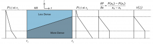
Since the pressure gradient can change with depth, the geostrophic current can change with depth. The vertical gradient of the geostrophic velocity is called the geostrophic shear. The diagram below shows a horizontal gradient in hydrostatic pressure that changes with depth due to a sloping surface of constant density, also called an isopycnal.
For the general case, where temperature and salinity vary continuously with depth, we can show mathematically that the geostrophic shear can be calculated from knowledge of just the density field. For example, starting with the east-west geostrophic velocity,
![\[ u =- \frac{1}{f \rho_0 }\frac{\partial P}{\partial y}, \]](https://uw.pressbooks.pub/app/uploads/quicklatex/quicklatex.com-b2b5de24e1a87733c408e904af71ee49_l3.png "Rendered by QuickLaTeX.com")
take the vertical derivative, and the swap the order of the partial derivatives to get
![\[ \frac{\partial u}{\partial z} =- \frac{1}{f \rho_0 }\frac{\partial }{\partial y}\frac{\partial P}{\partial z}. \]](https://uw.pressbooks.pub/app/uploads/quicklatex/quicklatex.com-eb48fbf9c816858dce288479d4218863_l3.png "Rendered by QuickLaTeX.com")
Next substitute in the hydrostatic vertical gradient of pressure to find the geostrophic shear in the x-direction
![\[ \frac{\partial u}{\partial z} =\frac{1}{f \rho_0 }\frac{\partial }{\partial y}(g \rho)\]](https://uw.pressbooks.pub/app/uploads/quicklatex/quicklatex.com-36fa202e3de64e035c198f25f4857bac_l3.png "Rendered by QuickLaTeX.com")
A similar derivation can be applied to the y-component of geostrophic velocity.
Key Takeaways
The geostrophic shear is related to horizontal gradients of density. For reasons related to their historical development in the atmosphere, these equations are called the thermal wind equations:
![\[ \frac{\partial u}{\partial z} =\frac{g}{f \rho_0 }\frac{\partial \rho}{\partial y} \]](https://uw.pressbooks.pub/app/uploads/quicklatex/quicklatex.com-749e1596cbc225b299d82280c6467a0c_l3.png "Rendered by QuickLaTeX.com")
![\[ \frac{\partial v}{\partial z} =-\frac{g}{f \rho_0 }\frac{\partial \rho}{\partial x} \]](https://uw.pressbooks.pub/app/uploads/quicklatex/quicklatex.com-8ebbbd5e8149ce8e80d0e478fe2a0248_l3.png "Rendered by QuickLaTeX.com")
Notes:
- The appropriate density to use when calculating the geostrophic shear is the potential density
- If you are feeling uncomfortable about swapping the order of the 2nd partial derivative between the first and second equations above (this is called a “mixed partial derivative” by the way), see the 2nd partial derivative article from Khan Academy.
Mini-lecture for class:
Media Attributions
- GeostrophicShear © Susan Hautala is licensed under a CC BY-NC-SA (Attribution NonCommercial ShareAlike) license
