28 Boundary layers

Since stress acts to diffuse momentum within the interior of a fluid, the shear is often relatively weak there.  At the boundary of the fluid domain, the velocity of the fluid must match the velocity of the surrounding material.  For example, the magnitude of the current flowing along the seafloor goes to zero right at the fluid-solid interface.  Often there is a layer of transition where the velocity gradient (the shear) can be very large.  This layer of transition is called a boundary layer.

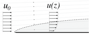
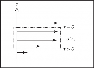
Historically, the mathematical development of boundary layers owes a lot to a the physical situation illustrated above, where a uniform and parallel (single component) flow enters the domain from the left edge and encounters an (infinitely thin, but zero velocity) plate. The width of the boundary layer grows with distance from the upstream edge as more of the fluid becomes affected by the diffusive flux of momentum toward the boundary where it is absorbed into the heat of molecular motion in the solid. You can understand this process by thinking about the control volume considered at the end of the last section (repeated below).  This control volume is on the edge of the boundary layer, and it is decelerated by the net frictional stress, creating shear near its lower surface, and leading to the propagation of the edge of the boundary layer into the fluid interior.

Boundary layers may also become turbulent, resulting in enhanced diffusion. The increased turbulent viscosity results in a larger stress for the same shear, and a more rapid thickening of the boundary layer with distance along the surface.

A boundary layer will also form near the surface of the ocean where the wind blowing across the surface creates a frictional stress on the air-sea interface.  This is similar to the moving top plate that we considered in the last section. We will return to the ocean’s surface boundary layer in a later section.