Introduction

Principal Coordinates Analysis (PCoA) is an unconstrained or indirect gradient analysis ordination method.  It was first published by Gower (1966).  The appealing element of PCoA is that it can be applied to semi-metric distance measures – those that do not satisfy the triangle inequality.  If it is applied to a metric distance measure, it functionally is identical to a PCA.

Confusingly, PCoA is also abbreviated PCO, and is also known as metric MultiDimensional Scaling (MDS).  Some authors distinguish PCoA from metric MultiDimensional Scaling (MDS) based on their numerical approach.  For example, Manly & Navarro Alberto (2017) state that PCoA is an eigenanalysis technique while MDS attempts to minimize stress.  However, others equate them – for example, the help files for cmdscale() state that the function performs classical multidimensional scaling (MDS), aka PCoA.  We won’t worry about these distinctions here.

For an example of how PCoA has been applied in an unusual context, see Metcalf et al. (2016)!

How PCoA Works

In a blog post (https://occamstypewriter.org/boboh/2012/01/17/pca_and_pcoa_explained/), Bob O’H provides a verbal description of the PCoA process, which I summarize here.

The goal of PCoA is to find a set of Euclidean distances that represent a set of non-Euclidean distances.  Borcard et al. (2018) describe PCoA as providing “a Euclidean representation of a set of objects whose relationships are measured by any dissimilarity measure chosen by the user” (p. 187).

If you only have two sample units, there is one distance to consider and therefore you can illustrate that distance on a (one-dimensional) number line.  If you have three sample units, there are also three distances to consider and illustrating these patterns will require one or two dimensions – either three points along a straight line or three points on a plane.  The general principle that this reflects is that n sample units can be illustrated or mapped in no more than n-1 dimensions.  

With this context, let’s summarize the PCoA procedure:

1. Place the first point at the origin.
2. Add the second point the correct distance away from the first point along the first axis.
3. Position the third point the correct distance away from each of the first two points, adding a second axis if necessary.
4. Position the fourth point the correct distance away from each of the first three points, adding another axis if necessary.
5. Continue until all points have been added.  The result is a set of no more than n-1 axes.
6. Conduct a PCA on the constructed points to organize the variation among the points in a series of axes of diminishing importance.

PCoA is intended for use with non-Euclidean distances and dissimilarities.   When applied to semi-metric distance measures (i.e., those that do not satisfy the triangle inequality), some of the resulting axes may be in ‘imaginary space’ (Anderson 2015).   These axes are mathematically possible but difficult to envision – you can’t graph them, for example.  When they are subject to PCA (see last step above), these imaginary axes produce negative eigenvalues. 

Two types of adjustments are possible that adjust the distance matrix to avoid negative eigenvalues:

• Lingoes correction – add a constant to the squared dissimilarities
• Cailliez correction – add a constant to the dissimilarities (Cailliez 1983)

Legendre & Anderson (1999) and Borcard et al. (2018) recommend using the Lingoes correction method but others use the Cailliez correction.  For example, in the RRPP chapter we noted that adonis2() and lm.rrpp() did not give the same results when applied to a Bray-Curtis distance matrix, and that this was because lm.rrpp() automatically makes this adjustment while adonis2() does not.  The author of the RRPP package noted that the outputs of the two functions agree if adonis2() uses the Cailliez correction method.  Making either of these adjustments has implications that I have not seen fully explored – see Appendix for one example.

Aside: if PCoA is applied to a set of Euclidean distances, it produces the same set of distances as in the original set and therefore does not change the distances.

Additional details about PCoA, and extensions to it, are provided in Anderson et al. (2008, ch. 3) and Borcard et al. (2018, ch. 5.5).

Similarities to PCA and NMDS

PCoA has similarities to both PCA and NMDS.

Like PCA…

Like PCA, PCoA is an eigenanalysis technique.  Manly & Navarro Alberto (2017; ch. 12.3) provide a detailed illustration of the connection between PCA and PCoA.  The fact that they are both eigenanalysis-based techniques means that:

• Points are projected onto axes.
• Since a PCA is the last step of a PCoA, the first axis necessarily explains as much of the variation as possible, the second axis explains as much of the remaining variation as possible, etc.
• As with PCA, PCoA is rotating and translating the data cloud.  If all axes are retained, no data reduction has occurred and the relative locations of the points to one another are unchanged.  This is true even when applied to non-Euclidean distances.
• The ‘fit’ of the PCoA can be assessed by the percentage of variation explained by each axis.

A PCoA using Euclidean distances is identical to a PCA of the same data.  Similarly, a PCoA using chi-square distances is identical to a CA of the same data (Anderson 2015).  In other words, PCA and CA are variants of PCoA, which is the more general technique.

Like NMDS…

Like NMDS, PCoA is a distance-based ordination technique and thus can be applied to any distance measure.  However, PCoA maximizes the agreement between the actual distances in ordination space and in the original space, whereas NMDS seeks only to maintain the rank order of the distances in the two matrices.  The help files for cmdscale() describes PCoA as returning “a set of points such that the distances between the points are approximately equal to the dissimilarities”.  Because of this focus on linear relationships, it has been suggested that PCoA is more appropriate than NMDS as an accompaniment to a PERMANOVA model (Anderson 2015).

PCoA in R (vegan::wcmdscale())

In R, PCoA can be accomplished using stats::cmdscale(), vegan::wcmdscale(), and ape::pcoa().  I’m sure other functions also exist for this purpose.

The wcmdscale() function is a wrapper that calls cmdscale() while providing some additional capabilities.  Its usage is:

wcmdscale(d,
k,
eig = FALSE,
add = FALSE,
x.ret = FALSE,
w
)

The arguments are:

• d – distance matrix to be analyzed.
• k – number of dimensions to save. Default is to save all non-negative eigenvalues (dimensions).  Up to n-1 eigenvalues are possible.
• eig – whether to save the eigenvalues in the resulting object. Default is to not do so (FALSE).
• add – whether to add a constant to the dissimilarities so that all eigenvalues are non-negative. Default is to not do this (FALSE) but two options are possible:
  • "lingoes" or TRUE – this is the option recommended by Legendre & Anderson (1999) and Borcard et al. (2018).
  • "cailliez" – this option is required for adonis2() results to match those from lm.rrpp().
• x.ret – whether to save the distance matrix. Default is to not do so.
• w – weights of points (sample units). If set to equual weights (w = 1; the default), this gives a regular PCoA.  If sample units are given different weights, those with high weights will have a stronger influence on the result than those with low weights.

The output of this function depends on the arguments selected.  If eig = FALSE and x.ret = FALSE, this returns just a matrix of coordinates for each positive eigenvalue.  Otherwise, this returns an object of class ‘wcmdscale’ with several components, including:

• points – the coordinates of each sample unit in each dimension (k).
• eig – the eigenvalue of every dimension. As noted above, some may be negative.
• ac – additive constant used to avoid negative eigenvalues. NA if no adjustment was made.
• add – the adjustment method used to avoid negative eigenvalues. FALSE if no adjustment was made.

An object of class ‘wcmdscale’ can be subject to pre-defined methods for print(), plot(), scores(), eigenvals(), and stressplot().

Oak Example

Use the ‘load.oak.data.R’ script to load our oak data and make our standard adjustments to it.

source("scripts/load.oak.data.R")

Now, apply a PCoA to our oak plant community dataset:

Oak1_PCoA <- wcmdscale(d = Oak1.dist, eig = TRUE)

Explore the output.  Try changing the k and eig arguments and see how the output changes (hint: str()).

print(Oak1_PCoA)

Call: wcmdscale(d = Oak1.dist, eig = TRUE)

          Inertia Rank
Total     11.5949     
Real      12.0707   34
Imaginary -0.4758   12

Results have 47 points, 34 axes

Eigenvalues:

 [1]  1.9133  1.2359  1.1947  0.8806  0.7649  0.6919  0.5303  0.4490
 [9]  0.4158  0.4001  0.3593  0.3388  0.3192  0.2857  0.2747  0.2413
[17]  0.2236  0.2012  0.1832  0.1670  0.1517  0.1384  0.1288  0.1112
[25]  0.1032  0.0880  0.0788  0.0552  0.0498  0.0354  0.0282  0.0157
[33]  0.0143  0.0014 -0.0021 -0.0102 -0.0124 -0.0240 -0.0295 -0.0334
[41] -0.0362 -0.0426 -0.0593 -0.0613 -0.0740 -0.0909

Weights: Constant

Note the presence of negative eigenvalues – in this case for 12 dimensions.  These are the additional dimensions that were required to fit the semi-metric Bray-Curtis distances into a Euclidean space.  However, the last step of the PCoA process was to conduct a PCA -this means that the coordinates have been rotated such that the axes are in descending order of importance.  Therefore, these dimensions account for small amounts of variation in the dataset.  If your objective is to reduce the dimensionality of the data, these dimensions can be ignored without changing your conclusions greatly.  Try changing the add argument and see how these are affected.

The output is a list as for metaMDS(), though this one isn’t as detailed.  The coordinates of the sample units are again reported as the points element within the list, though the axes are named differently than for a NMDS.  We’ll plot the first two axes using ggplot2.

ggplot(data = data.frame(Oak1_PCoA$points),
aes(x = Dim1, y = Dim2)) +
geom_point() +
theme_bw()

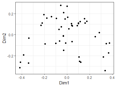
I displayed the axis coordinates here, but we could omit them to force the viewer to focus on the data cloud.  See the ‘Graphing the Final Configuration’ section from the NMDS chapter for an example of how to do so.

Uses of PCoA

We have already encountered PCoA several times:

• Displaying results of a PERMDISP analysis.
• Default option for generating the starting configuration for a NMDS.

Examples of other ways PCoA can be used:

• Combining functional traits of different organisms.  The FD package contains a dbFD() function that combines traits in different ways depending on their class and then combines the traits using PCoA (Laliberté & Legendre 2010).
• Expressing the location of centroids.  This is helpful, for example, when composition has been measured in multiple quadrats (sub-samples) per plot but where plots are the experimental units.  We could conduct a PCoA using the quadrats, keeping all dimensions.  Since these distances are now expressed in a Euclidean space, even if the original distance matrix was not, we can then calculate the centroid for each plot based on the locations of the quadrats in this ordination space.  The coordinates of these plots can then be the subject of statistical analysis.  An advantage of this approach is that it avoids the requirement of a balanced dataset for restricted permutations.  For example, you could calculate the centroid for each plot based on however many quadrats were sampled in that plot.

Interpreting PCoA

Since PCoA seeks to maximize the agreement between the actual distances in ordination space and in the original space, it is more similar to PERMANOVA than NMDS, which is based on the ranks of the distances.  Conceptually, therefore, the PCoA approach is more consistent with PERMANOVA, though I am not aware of any strong tests of this.  In addition, Anderson (2015) notes that NMDS generally works better than PCoA when visualizing a multi-dimensional distance matrix in a few dimensions.

As with PCA, keeping all axes means that the data cloud has been rotated but that its dimensionality has not been reduced.  This can be helpful, for example, because it allows you to express a non-Euclidean distance matrix in Euclidean units.  See the above section about ‘Uses of PCoA’ for examples.

Some people ‘object’ to the negative eigenvalues.  These are only an issue for distance measures that do not satisfy the triangle inequality.  Optional settings can be used to adjust the values so that no negative eigenvalues are produced (but see the Appendix for an illustration of how this adjustment can affect interpretation of results).  Even if these adjustments are not used, remember that if your purpose is data reduction, you are most interested in the first few dimensions – and those dimensions are rarely negative.

Conclusions

Several of these techniques are closely related.  For example, PCA and CA are applications of PCoA to particular types of distance measures.

The relative differences among some of these techniques are unclear; Anderson (2015) notes that techniques like NMDS and PCoA will all tend to give very similar results, and that far more important differences arise from decisions about data adjustments (transformations, standardizations) and which distance measure to use.

References

Anderson, M.J., R.N. Gorley, and K.R. Clarke. 2008. PERMANOVA+ for PRIMER: guide to software and statistical methods. PRIMER-E Ltd, Plymouth, UK.

Anderson, M.J. 2015. Workshop on multivariate analysis of complex experimental designs using the PERMANOVA+ add-on to PRIMER v7. PRIMER-E Ltd, Plymouth Marine Laboratory, Plymouth, UK.

Borcard, D., F. Gillet, and P. Legendre. 2018. Numerical ecology with R. 2nd edition. Springer, New York, NY.

Cailliez, F. 1983. The analytical solution of the additive constant problem. Psychometrika 48:305-308.

Gower, J.C. 1966. Some distance properties of latent root and vector methods used in multivariate analysis. Biometrika 53:325-338.

Laliberté, E., and P. Legendre. 2010. A distance-based framework for measuring functional diversity from multiple traits. Ecology 91:299-305.

Legendre, P., and M.J. Anderson. 1999. Distance-based redundancy analysis: testing multispecies responses in multifactorial ecological experiments. Ecological Monographs 69:1-24.

Manly, B.F.J., and J.A. Navarro Alberto. 2017. Multivariate statistical methods: a primer. Fourth edition. CRC Press, Boca Raton, FL.

Metcalf, J.L., Z.Z. Xu, S. Weiss, S. Lax, W. Van Treuren, E.R. Hyde, S.J. Song, A. Amir, P. Larsen, N. Sangwan, D. Haarmann, G.C. Humphrey, G. Ackermann, L.R. Thompson, C. Lauber, A. Bibat, C. Nicholas, M.J. Gebert, J.F. Petrosino, S.C. Reed, J.A. Gilbert, A.M. Lynne, S.R. Bucheli, D.O. Carter, and R. Knight. 2016. Microbial community assembly and metabolic function during mammalian corpse decomposition. Science 351(6269):158-162.