Contents

• Introduction
• The Indicator Value (IV)
• Groups or Combinations of Groups?
• Simplified ISA: Presence/Absence Data
• Published ISA Examples
• ISA in R (indicspecies::multipatt())
• Oak Example: Indicators of Grazing Treatments
• Additional Applications of ISA
• Recommendations for ISA
• What About TWINSPAN?
• Conclusions
• References
• PS: Graphs of Indicator Value Contours

Introduction

Indicator Species Analysis (ISA) was originally developed by Dufrêne & Legendre (1997) as a technique to identify species that are strongly associated with a particular group.  One motivation for developing this technique was to provide a tool for determining how many groups to focus on in a cluster analysis.

ISA is a remarkably simple technique that I think is underappreciated.  Advantages include:

• easy to calculate
• easy to interpret
• statistical significance is assessed via permutation tests
• can be used with any categorical classification (a priori or a posteriori)
• is calculated independently for each species

ISA has been extended in several ways since it was originally described:

• De Cáceres & Legendre (2009) showed how to use ISA to identify species that are associated with multiple groups.
• I (Bakker 2008) demonstrated that ISA produces very similar results if applied to presence/absence data rather than abundance data.  Implementation is identical, but with a matrix of presence/absence data instead of abundance data.
• In the same paper, I showed how ISAs from different sites can be combined.  I will not explore this idea further here, but it is available through indicspecies::signassoc().
• Baker & King (2010) developed TITAN to identify species that are associated with high or low values of a continuously distributed variable.

I will explain the way ISA was first proposed and how it was extended to multiple groups and to presence/absence data.  I consider TITAN separately.

The Indicator Value (IV)

ISA requires a typology, or classification of sample units into groups.

ISA involves calculating the specificity (A_ij; relative abundance) and fidelity (B_ij; relative frequency) of species i in group j.  The specificity and fidelity are then multiplied together to yield the test statistic, the Indicator Value (IV_ij).

where

• [latex]\bar{x}_{ij}[/latex] is the mean cover of species i within group j
• [latex]\sum_{j} \bar{x}_{i\bullet}[/latex] is the sum of the mean cover of species i in all groups
• [latex]n_{ij}[/latex] is the number of plots in group j occupied by species i
• [latex]n_{\bullet j}[/latex] is the total number of plots in group j.

Specificity is based on the mean covers in the various groups to account for potential differences in sample size among groups.  Species i has a specificity of 0 in group j if it is absent from the group, and has a specificity of 1 in group j if all of its abundance is in the group.

Species i has a fidelity of 0 in group j if it is absent from the group, and a fidelity of 1 in group j if it occurs in every plot within the group.

The key statistic is the Indicator Value (IndVal or IV or IV_ij).  Some notes about its interpretation:

• IV_ij is 0 when species i is absent from group j, and is at its maximum (1 or 100) when species i occurs on all plots within group j and does not occur in other groups.
• The highest IV_ij values occur for species that are common in one group and absent from other groups within the typology.
• Uncommon species will have low B_ij values and therefore low IV_ij values.
• Ubiquitous species (i.e., species present in all groups at a given level of the typology) have high B_ij values and therefore high IV_ij values.
• Dufrêne & Legendre (1997) suggest that species i be considered a ‘strong’ indicator of group j if IV_ij > 25.  There are multiple ways to arrive at this value.  For example:
  • If a species is present on at least 50% of the plots in group j (i.e., A_ij = 0.5) and also has at least 50% of its total abundance in group j (i.e., B_ij = 0.5)
  • If a species is present on at least 25% of the plots in group j (i.e., A_ij = 0.25) and also has all of its total abundance in group j (i.e., B_ij = 1.0)
  • If a species is present on all pots in group j (i.e., A_ij = 1.0) and also has at least 25% of its total abundance in group j (i.e., B_ij = 0.25)
• The minimum of IV_ij = 25 for a strong indicator as proposed by Dufrêne & Legendre (1997) is equivalent to IV_ij = 0.5 in the formulation reported by indicspecies::multipatt(), which takes the square root of this value.
• The figure below illustrates isoclines of IV:
  • Left: product of A_ij and B_ij (though expressed as a proportion rather than a percentage), as proposed by Dufrêne & Legendre (1997)
  • Right: squareroot of product of A_ij and B_ij, as reported by indicspecies::multipatt()

IV_ij is calculated for every species in every group, and each species i is tentatively considered an indicator of the group j in which its IV is largest.  The statistical significance of these values is assessed using permutation tests.  These tests are necessary because ubiquitous species have high IV_ij values but are not helpful in distinguishing one group from another.

Groups or Combinations of Groups?

The classical ISA considers groups individually: each species can be an indicator of one group.  For example, imagine that you were comparing samples from forest, grassland, and river.  The classical ISA could identify species that are indicators of forest OR grassland OR river.  A species that occurred in both forest AND grassland might not be identified as an indicator of either habitat.

Miquel De Cáceres and colleagues (De Cáceres & Legendre 2009; De Cáceres et al. 2010) extended the classical ISA to enable the identification of indicators of combinations of groups.  They argued that this extension provides a way to identify species with differing niche breadths (i.e., niches spanning more than one category).  For example, in the habitat example described above, the method proposed by De Cáceres et al. tests for indicators of individual habitats (forest OR grassland OR river) and for indicators of combinations of habitats (e.g., (forest + grassland) OR river).

You can test all possible combinations or restrict attention to those combinations of groups that make ecological or statistical sense.  What would not make ecological sense?  For example, in the above habitat example, it seems reasonable to consider forest and grassland together since they are both terrestrial habitats that a species with a wide ecological niche could occupy, but it would not make sense to combine forest and river together.  What would not make statistical sense?  If you had conducted a hierarchical cluster analysis, the groups are fused together in the structure summarized in a dendrogram.  It would not make sense to combine groups that were created in different branches of the tree.  In other words, the cluster groups that are considered should reflect the hierarchical nature of the dendrogram.

The restcomb argument within indicspecies::multipatt() provides control over which combinations are considered.

Simplified ISA: Presence/Absence Data

Dufrêne & Legendre (1997) also proposed a simplified ISA based on presence/absence data.  For the simplified ISA, the formula for specificity (A_ij) is modified to:

[latex]A_{ij} = \frac {n_{ij}}{n_{i\bullet}}[/latex]

where

• [latex]n_{ij}[/latex] is the number of plots in group j occupied by species i
• [latex]n_{i\bullet}[/latex] is the total number of plots occupied by species i

Verbally, specificity is now the proportion of plots occupied by species i that are located in group j.  Fidelity (B_ij) and IV_ij are calculated as above.

In practice, a simplified ISA can be implemented by transforming the data to binary data (i.e., 0 = absence, 1 = presence) and calculating the ISA on the transformed data.

If a species is equally abundant on all plots where it occurs, the classical and simplified ISAs yield identical results.  As variability in abundance among plots increases, the classical and simplified ISAs give differing weights to A_ij, and therefore yield different results.

A potentially large advantage of the simplified ISA is that the data are easily summarized and displayed.  To summarize the data necessary for the classical ISA, you need the raw data (i.e., abundance of species i on every plot j) or at least the mean abundance of species i in every group j.  In contrast, the data needed for the simplified ISA can be succinctly summarized.  The above formulae require only three values to calculate the simplified ISA for a given species:

• [latex]n_{ij}[/latex] = the number of plots in group j occupied by species i
• [latex]n_{i\bullet}[/latex] = the total number of plots occupied by species i
• [latex]n_{\bullet j}[/latex] = the total number of plots in group j

The simplified ISA can be conducted using the classical approach (each group separately) or the extension to combinations of groups.

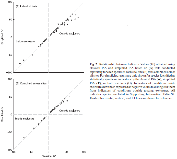
In an earlier study (Bakker 2008), I used classical (abundance-based) and simplified (presence/absence-based) ISAs to identify indicators of grazing treatment.  There were 206 unique tests, each consisting of one species at one site.  This study found (based in part on the below figure):

• In 94% (193 of 206) of tests, the classical and simplified ISAs identified the same grazing treatment as having the maximum IV.
• In no test did the two methods identify opposite grazing treatments as statistically significant indicators.
• Overall, 62 species were identified as statistically significant indicators of grazing treatment.  Of these:
  • 85% (53 of 62) were identified by both methods
  • 13% (8 of 62) were identified by the classical ISA only
  • 2% (1 of 62) were identified by the simplified ISA only

Published ISA Examples

Zald et al. (2020) identified plant species associated with different seasons and intervals of burning.

Pillsbury et al. (2019) used ISA to identify diatoms associated with high and low nitrogen and phosphorus conditions.

Martin & Hamman (2016) used ISA to identify the fire severity class associated with each of several plant life forms.

Severns & Sykes (2020) propose that phytopathologists use ISA to identify the fungi associated with plant diseases.

ISA in R (indicspecies::multipatt())

There are several functions that can conduct ISA in R.  They vary in some details, such as how IV is reported.  We will focus on indicspecies::multipatt() but others include labdsv::duleg() and adiv::dbMANOVAspecies() (Ricotta et al. 2021).

The usage of multipatt() is:

multipatt(
x,
cluster,
func = "IndVal.g",
duleg = FALSE,
restcomb = NULL,
min.order = 1,
max.order = NULL,
allow.negative = FALSE,
control = how(),
permutations = NULL,
print.perm = FALSE
)

The key arguments are:

• x – the plot x species data table
• cluster – a vector consisting of the group to which each plot belongs.  Although this is called ‘cluster’, the groups do not have to come from a cluster analysis.
• func – function to calculate the strength of the association of each species with the groups.  Options are "IndVal", "IndVal.g", "r", and "r.g".  IndVal and IndVal.g are the IV mentioned above, while r and r.g are correlations.  The ‘.g’ suffix indicates that they include a correction for sample sizes, and are the recommended functions to use.  IndVal.g is the default.
• duleg – whether to consider groups of sites (FALSE; default) or not (TRUE).  Argument name is an abbreviation of Dufrêne & Legendre (1997), who only considered indicators of individual sites.  If duleg = TRUE, this conducts the classical ISA that they originally proposed.
• restcomb – a vector of integers that restricts attention to combinations of groups that make ecological sense to the analyst.  Not applicable if doing a classical ISA.  Conduct analysis using all groups (default settings for duleg, min.order, and max.order), and view the resulting object to find the integer associated with each combination of groups.
• min.order – minimum number of sites (i.e., levels of a factor) to include in groups of sites.  Default is 1 (i.e., individual sites can be their own groups).
• max.order – maximum number of sites (i.e., levels of a factor) to include in groups of sites.  For example, if max.order = 2, then two levels can be combined into a group but a group including three levels will not be tested.
• allow.negative - whether to allow negative associations.  Only possible for func = "r" or func = "r.g".
• control – options for controlling how permutations are conducted.  This uses the same permute::how() function that we saw in our group comparison methods.

The resulting object is of class 'multipatt' with several elements, including:

• comb – a plot x combination matrix, with a column for every combination of groups tested. The values within this matrix are 1 if that plot is included in that combination of groups and 0 otherwise.  The column number is the integer value by which these combinations are referenced in other elements.
• A – a species x combination matrix, with a column for every combination of groups tested.  The values are the specificity component of IV for that species in that combination of groups.
• B – a species x combination matrix, with a column for every combination of groups tested.  The values are the fidelity component of IV for that species in that combination of groups
• sign – a data table summarizing the results for each species:
  • The ‘index’ column contains an integer denoting the combination of groups in which the species had its maximum IV.
  • The ‘stat’ column reports the square root of the IV.  The column has a generic name because it can also return correlations (func = "r" or func = "r.g").
  • The ‘p.value’ column reports the permutation-based p-value associated with stat.  Note that there is no p-value when the maximum IV is in the largest combination of groups (i.e., all plots in a single group) as there are no permutations possible.

Applying summary() to the resulting object focuses on those species that meet desired criteria.  The default is to show those species that are statistically significant at alpha = 0.05.  Setting the indvalcomp argument to TRUE returns the specificity and fidelity in addition to the IV.  See ?summary.multipatt for details of other criteria.

One caution about only viewing statistically significant taxa is that the p-value is permutation-based and therefore can vary between runs; species may be identified as significant indicators in one run but not in another run.  To avoid this issue, use a set group of permutations (set.seed()).

Oak Example: Indicators of Grazing Treatments

In the introductory material of this section, we demonstrated that there is a statistically significant difference in composition between the three grazing treatments.  Let’s see which species are strongly associated with one grazing status over the others.  We will do this using the three approaches described above: classical ISA (i.e., each group distinct), ISA allowing combinations of groups, and simplified ISA (with combinations of groups).

To ensure that results are directly comparable amongst analyses, we will use the same set of permutations in each analysis.

Classical ISA

To use the classical ISA, we specify x and cluster, and include the argument ‘duleg = TRUE’:

library(indicspecies)

set.seed(42)

Graz.ISA <- multipatt(x = Oak1,
cluster = Oak_explan$Grazing,
duleg = TRUE)

summary(Graz.ISA, indvalcomp = TRUE)

Multilevel pattern analysis
---------------------------

Association function: IndVal.g
Significance level (alpha): 0.05

Total number of species: 103
Selected number of species: 6 
Number of species associated to 1 group: 6 
Number of species associated to 2 groups: 0 

List of species associated to each combination: 

Group Always  #sps.  2 
          A      B stat p.value  
Popr 0.8466 0.6471 0.74    0.04 *
Agte 0.7348 0.7059 0.72    0.03 *

Group Never  #sps.  2 
            A      B  stat p.value   
Prav.s 0.8788 0.7917 0.834   0.005 **
Syal.s 0.5734 1.0000 0.757   0.005 **

Group Past  #sps.  2 
            A      B  stat p.value  
Rhdi.s 0.4763 1.0000 0.690   0.015 *
Aqfo   0.8889 0.3333 0.544   0.035 *
---
Signif. codes:  0 ‘***’ 0.001 ‘**’ 0.01 ‘*’ 0.05 ‘.’ 0.1 ‘ ’ 1 

Six of the 103 species are identified as significant indicators.  All such indicators are associated with a single group (no other options are possible with the classical ISA).  In this case:

• Popr and Agte are indicators of always grazed stands
• Prav.s and Syal.s are indicators of never grazed stands
• Rhdi.s and Agfo are indicators of stands that were grazed only in the past

Note that it is simply chance that there are equal numbers of indicators for each grazing treatment.  There could easily be uneven numbers of indicators, and groups for which no indicators are identified.

Each species is identified by the unique code that named its column.  We can use these codes to look their names in our Oak_spp object and then draw on our ecological knowledge of the system to interpret them.

ISA with Combinations of Groups

Our grazing example includes three levels that can be combined into seven groups:

(these combinations of groups are identified in Graz.ISA.2$comb below)

The multipatt() function automatically combines the levels of our grouping variable into groups of levels.  We can use the restcomb argument to restrict our attention to particular combinations of groups.  For example, we might decide that the group ‘Always+Never’ is ecologically questionable and therefore exclude it from consideration (I have not done so here, however).

ISA with multiple groups is the default in multipatt():

set.seed(42)

Graz.ISA.2 <- multipatt(x = Oak1,
cluster = Oak_explan$Grazing)

summary(Graz.ISA.2, indvalcomp = TRUE)

Multilevel pattern analysis
---------------------------

Association function: IndVal.g
Significance level (alpha): 0.05

Total number of species: 103
Selected number of species: 9 
Number of species associated to 1 group: 1 
Number of species associated to 2 groups: 8 

List of species associated to each combination: 

Group Past  #sps.  1 
          A      B  stat p.value  
Aqfo 0.8889 0.3333 0.544   0.035 *

Group Always+Past  #sps.  6 
          A      B  stat p.value   
Sado 0.8135 0.8696 0.841   0.005 **
Popr 0.9396 0.6957 0.808   0.010 **
Elgl 0.7886 0.7826 0.786   0.030 * 
Hola 0.8688 0.6522 0.753   0.035 * 
Agte 0.8674 0.6087 0.727   0.045 * 
Acmi 0.9393 0.3913 0.606   0.015 * 

Group Never+Past  #sps.  2 
            A      B  stat p.value  
Prav.s 0.9526 0.8000 0.873   0.015 *
Ronu.s 0.9328 0.5333 0.705   0.045 *
---
Signif. codes:  0 ‘***’ 0.001 ‘**’ 0.01 ‘*’ 0.05 ‘.’ 0.1 ‘ ’ 1

In this analysis, 9 of the 103 species are identified as indicators.  One indicator is associated with an individual group, and the others are associated with combinations of groups.  In this case there are:

• One indicator (Agfo) of stands that were only grazed in the past
• Six indicators (Sado, Popr, Elgl, Hola, Agte, and Acmi) of stands that were either always grazed or only grazed in the past (i.e., not never grazed)
• Two indicators (Prav.s, Ronu.s) of stands that were not currently grazed (i.e., either Never or Past grazed)

Allowing for indicators to be identified across multiple groups has changed some of the indicators.  For example, there are no indicators of stands that were only Never grazed whereas in the above analysis two species were indicators of this group.  Aqfo is still identified as an indicator of a single group (Past), so its test statistic is identical here to what was calculated with the Classical ISA.

Simplified ISA (Presence/Absence Data)

To analyze these data using presence/absence data, we need to relativize the data in that way first.  We’ll use the multi-group ISA here.

Oak1.pres <- decostand(Oak1, "pa")

set.seed(42)

Graz.ISA.pres <- multipatt(x = Oak1.pres,
cluster = Oak_explan$Grazing)

summary(Graz.ISA.pres, indvalcomp = TRUE)

Multilevel pattern analysis
---------------------------

Association function: IndVal.g
Significance level (alpha): 0.05

Total number of species: 103
Selected number of species: 8 
Number of species associated to 1 group: 2 
Number of species associated to 2 groups: 6 

List of species associated to each combination: 

Group Past  #sps.  2 
            A      B  stat p.value  
Frla.s 0.6375 0.5000 0.565   0.050 *
Aqfo   0.8889 0.3333 0.544   0.035 *

Group Always+Past  #sps.  6 
          A      B  stat p.value   
Sado 0.8547 0.8696 0.862   0.005 **
Brla 0.7802 0.9130 0.844   0.005 **
Elgl 0.7932 0.7826 0.788   0.020 * 
Popr 0.8555 0.6957 0.771   0.005 **
Acmi 0.9470 0.3913 0.609   0.010 **
Cyec 1.0000 0.2609 0.511   0.030 * 
---
Signif. codes:  0 ‘***’ 0.001 ‘**’ 0.01 ‘*’ 0.05 ‘.’ 0.1 ‘ ’ 1 

Eight of the 103 species are identified as indicators.  Two species are indicators of one group, and the others are indicators of a combinations of two groups.  In this case there are:

• Two indicators (Frla.s, Agfo) of stands that were only grazed in the past
• Six indicators (Sado, Brla, Elgl, Popr, Acmi, and Cyec) of stands that were either always grazed or only grazed in the past (i.e., not never grazed)

Results based on presence/absence data are broadly similar to, but not identical, to those in where we considered combinations of groups but also incorporated species abundance information.

Summarizing ISA Results

An interesting element is to compare analyses and identify which indicators have changed in status.  This can be done on the basis of the magnitude and significance of IV.  Here, we’ll just focus on those species that were identified as significant indicators and compare these across the three ISAs that we conducted.  I’ve sorted this list alphabetically by species code.

Some observations:

• Aqfo was a consistent indicator of the same group (Past) regardless of how the analysis was conducted.
• Several species that were identified as indicators of a single group in the classical ISA were determined to be even stronger indicators of a combination of groups in the multiple group and/or simplified ISAs.
• Several species were not identified as indicators of a single group in the classical ISA but were identified as strong indicators of a combination of groups in the other analyses.
• Species that were identified as significant indicators in the multiple group ISA but not in the simplified ISA differ more strongly in abundance among groups.
• None of the shrubs (species codes ending in ‘.s’) were indicators of stands that were currently grazed (Always), perhaps reflecting their sensitivity to livestock.
• Indicators of the ‘Never’ and ‘Always’ groups were only detected in the Classical ISA; most of these species were more strongly associated with a combination of groups in the other analyses.

The complete results for each analysis include all species regardless of their statistical significance – we could look at this to see which combination they were most strongly associated with.

Additional Applications of ISA

Hierarchical Analyses

Dufrêne & Legendre’s (1997) original description of ISA was as a method to identify how many groups to focus on in a hierarchical cluster analysis.  For example, they identified the number of groups in the cluster analysis at which each species achieved its largest IV, and then tallied those up – the height in the dendrogram that produced the greatest number of largest IVs was adopted as the solution and those groups were chosen.

The hierarchical structure of a dendrogram can be easily incorporated into the multi-group ISA (restcomb argument), combining groups in the order that they are fused in the dendrogram, and omitting those that are not supported by the dendrogram.

Non-Hierarchical Analyses

Not all data have a hierarchical typology.  For example, if you were interested in two explanatory variables, you could conduct an ISA for each of them and then combine the results.

In one project, I was interested in indicators of overstory condition (either in the open or under tree canopy) and of grazing treatment (inside or outside livestock exclosures).  I did an ISA with each type of grouping, and then organized species based on their responses - some representative species are shown here:

Observations:

• Species such as Sporobolus interruptus and Bromus tectorum were indicators of different types of overstory condition but were not indicators of grazing treatment.  These species may be more sensitive to the light environment than to grazing-related disturbances.
• Species such as Elymus elymoides and Muhlenbergia montana were indicators of different grazing treatments but were not indicators of overstory condition.  These species may be more sensitive to grazing but can occur under a wide range of light environments.
• Species such as Achillea millefolium, Trifolium longipes, Hesperostipa comata, and Festuca arizonica were indicators of both overstory condition and grazing treatment.  These species may have narrower ecological niches that are influenced by both factors.  Each species was an indicator of a different combination of these factors.
• Some species (not identified in table) were not indicators of either factor.

Comparisons like this can be more ecologically nuanced than just thinking about a single factor. For example, they reflects the fact that different factors shape the distributions of different species.

Consistency of Indicators Among Sites

One aspect of ISA that hasn’t received much attention to date is the consistency of indicators across replicate sites or studies.  Meta-analytical techniques can be used to combine the ISA results from multiple sites and thereby assess the consistency of indicators (see Bakker 2008 for details).

For example, areas inside and outside a grazing exclosure at each of five sites in northern Arizona were sampled in 1941.  I used these data to examine whether Muhlenbergia montana, a common grass, was an indicator of conditions inside or outside livestock exclosures.  To do so, I analyzed each site separately and then combined the results into an overall value for each grazing treatment:

M. montana was clearly not a statistically significant indicator of conditions inside exclosures at one site and was marginally significant at a second site, but was a significant indicator of these areas at three other sites.  When considered together, it was clearly an indicator of conditions inside exclosures overall.  I did similar analyses with a number of other species and found that species that occurred on multiple sites were more likely to be indicators than those that occurred on a single site.

Meta-Analyses

Since ISA is calculated separately for each species, the data can also be summarized separately for each species - for example, there is no need to keep track of which plot each species occurred in.  This is particularly useful for the simplified ISA, which only requires three values as noted above.

If the relevant data are reported in the literature, they can be used to assess the generality of indicator species using independent datasets.  Furthermore, since ISAs are conducted independently for each species, studies of commonly studied factors can be drawn from across the distributional range of each species (Bakker 2008).

Species Combinations

De Cáceres et al. (2012) proposed that ISA could also be used to identify combinations of species that distinguish sites.  This might occur, for example, if two species are functionally equivalent or even if a taxon was identified to the species level in some plots but to the genus level in other plots (e.g., Poa pratensis, Poa spp.).

This approach can be implemented using indicspecies::combinespecies() to create combinations of species, up to some max.order.  See De Cáceres (2025) for details.

Recommendations for ISA

Some recommendations for using ISA, particularly with respect to the potential to combine the results of multiple sites or studies:

1. When collecting data, identify individuals to the finest taxonomic level possible. Congeneric species, for example, may differ in indicator status (Weiss & Rice 2005; Nahmani et al. 2006) and may differ in nativity and other characteristics.
2. Consider the proper exchangeable units for the permutations tests (Anderson & ter Braak 2003). Where appropriate, such as when a factor is nested within sites, sites can be analyzed separately and the results combined using meta-analytic techniques (Bakker 2008).
3. Comparisons of ISAs from multiple studies require that the same typology be used in each study. Simple pairwise comparisons (e.g., grazed vs. ungrazed) are more likely to be comparable between studies than comparisons among multiple levels. Groups included in the typology should be described in detail.
4. Ensure that the sample size within each group is sufficient to sample the vegetation. Doing so will also provide enough samples to permit an adequate number of permutations for assessing statistical significance.
5. At a minimum, report the sample size and frequency of all species in all groups, so that the simplified IV can be calculated. Digital appendices and other repositories permit the archiving of these data in an accessible manner (Parr & Cummings 2005).
6. To prevent publication bias in future meta-analyses (Gurevitch & Hedges 2001), publish data for all species, regardless of whether or not they were significant indicators.

What about TWINSPAN?

Prior to the development of ISA, the main statistical technique for identifying species associated with groups was Two-Way INdicator SPecies ANalysis (TWINSPAN) (Hill et al. 1975; McCune & Grace 2002, ch. 12).  TWINSPAN is a divisive approach – it starts from the assumption that everything is in one group and then looks for ways to divide that group.  However, several aspects of TWINSPAN greatly limit its utility:

• cannot be used for predefined groups
• performs poorly with > 1 gradient
• involves complex analytical details
• is based on Correspondence Analysis (CA) and therefore on chi-square distances
• requires “pseudospecies” to convert quantitative abundance data into qualitative presence/absence data (place abundances into classes and consider each class equivalent to a pseudospecies)

I have not seen TWINSPAN used in recent years.

Conclusions

ISA is an extremely powerful technique.  It has high applicability for identifying species that differ between groups.

ISA differs from SIMPER in several ways.  First, ISA provides more guidance about species that differ: if a species is an indicator of one group over the other we know that it is more abundant and frequent in the first group.  In contrast, SIMPER quantifies how much a species contributes to the difference between groups but doesn't indicate where the species occurs.  Second, all sample units are considered simultaneously in ISA whereas the contribution of each species to each pairwise distance is calculated in SIMPER and then those contributions are averaged.  This means that the connection to the actual dissimilarity between sample units is not as strong for ISA, though I have not seen explicit comparisons of ISA and SIMPER.  However, they can be complimentary - for example, you could use ISA to identify indicator species between two groups and then use SIMPER to quantify how much of the variation between those groups is accounted for by the indicator species.

ISA was not designed to relate species to continuously distributed explanatory variables, though it has been adapted for that purpose as part of a technique known as TITAN.

Data adjustments remain important; these calculations will be affected by adjustments.  You should use the same adjustments as in all other aspects of your analysis.

References

Anderson, M.J., and C.J.F. ter Braak. 2003. Permutation tests for multi-factorial analysis of variance. Journal of Statistical Computation and Simulation 73:85-113.

Baker, M.E., and R.S. King. 2010. A new method for detecting and interpreting biodiversity and ecological community thresholds. Methods in Ecology and Evolution 1:25-37.

Bakker, J.D. 2008. Increasing the utility of Indicator Species Analysis. Journal of Applied Ecology 45:1829-1835.

De Cáceres, M., and P. Legendre. 2009. Associations between species and groups of sites: indices and statistical inference. Ecology 90:3566-3574.

De Cáceres, M., P. Legendre, and M. Moretti. 2010. Improving indicator species analysis by combining groups of sites. Oikos 119:1674-1684.

De Cáceres, M., P. Legendre, S.K. Wiser, and L. Brotons. 2012. Using species combinations in indicator value analyses. Methods in Ecology and Evolution 3:973-982.

De Cáceres, M. 2025. Indicator Species Analysis using 'indicspecies'.

Dufrêne, M., and P. Legendre. 1997. Species assemblages and indicator species: the need for a flexible asymmetrical approach. Ecological Monographs 67:345-366.

Gurevitch, J., and L.V. Hedges. 2001. Meta-analysis: combining the results of independent experiments. Pages 347-369 in S.M. Scheiner and J. Gurevitch (editors). Design and Analysis of Ecological Experiments. Oxford University Press, New York, NY.

Hill, M.O., R.G.H. Bunce, and M.W. Shaw. 1975. Indicator Species Analysis, a divisive polythetic method of classification, and its application to a survey of native pinewoods in Scotland. Journal of Ecology 63(2):597-613.

Martin, R.A., and S.T. Hamman. 2016. Ignition patterns influence fire severity and plant communities in Pacific Northwest, USA, prairies. Fire Ecology 12:88-102.

McCune, B., and J.B. Grace. 2002. Analysis of Ecological Communities. MjM Software Design, Gleneden Beach, OR.

Nahmani, J., P. Lavelle, and J.-P. Rossi. 2006. Does changing the taxonomic resolution alter the value of soil macroinvertebrates as bioindicators of metal pollution? Soil Biology and Biochemistry 38:385-396.

Parr, C.S., and M.P. Cummings. 2005. Data sharing in ecology and evolution. Trends in Ecology and Evolution 20:362-363.

Pillsbury, R.W., R.J. Stevenson, M. Munn, and I.R. Waite. 2019. Relationships between diatom metrics based on species nutrient traits and agricultural land use. Environmental Monitoring and Assessment 191:228.

Ricotta, C., S. Pavoine, B.E.L. Cerabolini, and V.D. Pillar. 2021. A new method for indicator species analysis in the framework of multivariate analysis of variance. Journal of Vegetation Science 32(2):e13013.

Severns, P.M., and E.M. Sykes. 2020. Indicator Species Analysis: a useful tool for plant disease studies. Phytopathology 110(12):1860-1862.

Smucker, N.J., E.M. Pilgrim, C.T. Nietch, J.A. Darling, and B.R. Johnson. 2020. DNA metabarcoding effectively quantifies diatom responses to nutrients in streams. Ecological Applications 30:e02205.

Weiss, J.M., and S.R. Reice. 2005. The aggregation of impacts: using species-specific effects to infer community-level disturbances. Ecological Applications 15:599-617.

Zald, H.S.J., B.K. Kerns, and M.A. Day. 2020. Limited effects of long-term repeated season and interval of prescribed burning on understory vegetation compositional trajectories and indicator species in ponderosa pine forests of northeastern Oregon, USA. Forests 11:834.

PS: Graphs of Indicator Value Contours

Here's the code to create the above figure showing contours for Indicator Value based on different values for A_ij and B_ij.

temp <- expand.grid(Aij = seq(0, 1, 0.01),
Bij = seq(0, 1, 0.01))

temp <- temp %>%
mutate(IVij = Aij * Bij,
sqrt.IVij = sqrt(IVij))

IV.graph <- ggplot(data = temp,
aes(x = Aij, y = Bij, z = IVij)) +
geom_contour_filled() +
geom_contour(colour = "black") +
labs(title = "IndVal",
x = "Specificity (Aij)",
y = "Fidelity (Bij)") +
theme_bw() +
theme(text = element_text(size = 9))

sqrt.IV.graph <- ggplot(data = temp,
aes(x = Aij, y = Bij, z = sqrt.IVij)) +
geom_contour_filled() +
geom_contour(colour = "black") +
labs(title = "squareroot(IndVal)",
x = "Specificity (Aij)",
y = "Fidelity (Bij)") +
theme_bw() +
theme(text = element_text(size = 9))

ggarrange(IV.graph, sqrt.IV.graph, common.legend = TRUE)

ggsave("graphics/IndVal.contours.png",
width = 5, height = 3, units = "in", dpi = 600)