
Foundational Concepts
4 R Basics
Learning Objectives
To understand the object-oriented nature of R, including object names and classes.
To understand how objects can be manipulated via operators and indexing.
To introduce ways to combine functions via nested functions and piping.
To introduce the tidyverse and other ways to manipulate data, including combining objects.
Resources
Manly & Navarro Alberto (2017, ch. 1)
RStudio cheat sheets for reference:
- RStudio IDE
- Base R
- Data Import with
readr,readxl, andgooglesheets4 - Apply Functions with purrr
- Data Tidying with
tidyr - Data Transformation with
dplyr - Data Visualization with
ggplot2 - Dates and times with
lubridate - Factors with
forcats - String Manipulation with
stringr - Cheat Sheet::VEGAN
- Git and GitHub with RStudio
- Other cheat sheets available at https://posit.co/resources/cheatsheets/
Key Packages
tidyverse, plyr
Introduction
If you are new to R, you might find it helpful to read the brief “Field Guide to the R Ecosystem” (Sellors 2019), which introduces the main components of the R ‘ecosystem’. Robinson (2016) also summarizes the key aspects of R in his “icebreakeR”. If you are familiar with SAS or SPSS, you may find the ‘Quick-R’ website particularly helpful.
For an introduction to the basic instructions about R, see the appendix to chapter 1 of Manly & Navarro Alberto (2017), chapter 1 of Dalgaard (2008), Paradis (2005; sections 2-3; online), and Torfs & Brauer (2014). Somewhat more advanced references include Adler (2010) and Borcard et al. (2018). Finally, very comprehensive reference materials are provided in the official R manual by Venables et al. (2023) and in many other publications, including Crawley (2012), Wickham (2014), and Wickham & Grolemund (2017).
For day-to-day reminders when using R, cheatsheets such as those linked to above can be very helpful.
Assigning Names
By convention, R code is displayed in a different font than regular text.
Name objects by assigning them to a name:
name <- object
R is Object Oriented
R is object oriented. This means that each variable, dataset, function, etc. is stored as an object. Each object is named, and can be manipulated.
Objects are created by assigning them to a name. When naming objects, there are a few conventions to keep in mind:
- Must begin with a letter (A-Z, a-z)
- Can include letters, digits (0-9), dots (.), and underscores (_)
- Are case-sensitive –
nandNare different objects - No size limits that I know of. You can create long and descriptive names for your objects … but you’ll have to type them out every time you need to call them.
- If you specify an object that already exists, the existing value assigned to that name is over-written without warning
Although there is considerable flexibility in how objects are named, consistency is very helpful. Some key recommendations are provided in the textbox below.
Naming Conventions
The Tidyverse Style Guide (Wickham 2020) recommends:
- Use only lowercase letters, numbers, and the underscore (_) when naming variables and functions.
- Use the underscore to separate words within a name. For example,
day_onerather thandayone. - Use nouns for variable names and verbs for function names.
- Avoid the names of common functions and variables. For example, if you named your data object as
datait would easily be confused with thedata()function.
Operators
Objects are manipulated via operators and functions (other objects). Common operators include:
| Operator | Description |
| Mathematical | |
+ - |
Addition, Subtraction |
* / |
Multiplication, Division |
^ |
Exponentiation |
| Relational | |
<- = |
Assignment: items to right of operator are assigned to name on left of operator. While these operators are synonymous, ‘<-’ is recommended because it can only be used in assignment while ‘=’ can be used in many other situations. ?assignOps for details. |
-> |
Rightwards assignment: items to left of operator are assigned to name on right of operator |
== |
Test of equality |
!= |
Not equal to |
< |
Less than |
<= |
Less than or equal to |
> |
Greater than |
>= |
Greater than or equal to |
| Logical | |
& && |
And |
| || |
Or |
! |
Not |
?Syntax for details about many of these operators, including their precedence (the order in which they are evaluated).
If you type in an expression but don’t assign it to a name, the result will be displayed on the screen but will not be stored as an object in memory. For example:
2 + 3 # Result not stored in memory
n <- 2 + 3
n
n + 3
Do you see the difference? This is a trivial example because it involves a single number, but the principle holds even with complex analyses (e.g., of objects that consist of many elements). Here is a random sample of 100 observations from a standard normal distribution (i.e., with mean = 0 and standard deviation = 1):
N <- rnorm(100)
Now that all of these elements have been assigned to the object N, they can be manipulated en masse. To multiply each of these random samples by 2:
2 * N
How would we save these new numbers to an object?
We could also calculate the average of these random samples:
mean(N)
Your mean value should not match mine exactly. Why not?
Multiple commands can be written on a single line if separated by semi-colons. This can be helpful to save space in a program script. For example, we assigned the result of adding 2 and 3 to the object n above, but this result wasn’t displayed on the screen until we requested it. We could do both functions on a single line, separated by a semi-colon:
n <- (4 * 5) / 2; n # Note that we’ve now reassigned ‘n’ to a new object!
We can also wrap a function in parentheses to simultaneously execute it and display it on the screen:
(m <- 1:10)
Comments
Functions can be annotated by adding comments after a #. Anything from the # to the end of the line is ignored by R.
Comments are useful for annotating code, such as explaining what a line does or what output is produced. For example, I often use a comment to document the dimensionality of an object – this gives me a quick way to check that the code is producing an object of the correct size when I rerun it. However, some argue that comments should be used minimally as they easily become out-of-date and can therefore be confusing when checking code (Filazzola & Lortie 2022).
Comments can also be helpful when writing larger pieces of code, as you can selectively turn lines of code off or on by adding or removing a # from the front of the line. In RStudio, you can apply this to multiple lines at once by highlighting those lines and selecting ‘Code -> Comment/Uncomment Lines’.
In the RStudio editor pane, comments are displayed in a different color than non-commented code.
Object Classes
Every object in R belongs to one or more classes. Classes have distinct attributes which control what type(s) of data an object can store, and how those objects may be used. Many functions are built to only work for objects of a specified class. The help file for a function will often specify which class(es) of object it works on.
| Class | Description |
numeric |
One-dimensional. ‘Regular’ numbers (e.g., 4.2). |
integer |
One-dimensional. Whole numbers (e.g., 4). |
character |
One-dimensional. Text (e.g., four). |
matrix |
Two-dimensional. All data within an array must be of the same type. |
array |
Multi-dimensional. All data within an array must be of the same type. |
data.frame |
Two-dimensional; resembles a matrix, but data within different columns (vectors) may be of different types. Data within a given column must be of the same type, and all columns must be of the same length. This is one of the most flexible and common ways of storing data. |
list |
Multi-dimensional; similar to a data frame but the ‘columns’ do not have to be the same length. The objects that result from R functions are often stored as lists. |
factor |
A collection of items. Can be character (forest, prairie) or numerical (1, 2, 3). If specified as explanatory variables in an analysis, character data are often recognized as factors and treated appropriately, but numerical data may be assumed to be continuous and treated as covariates unless specified as a factor. If the levels are ordinal (e.g., low, medium, high), the correct ordering can be specified. |
logical |
Binary (True/False). Often used to index data by identifying data that meet specified criteria. |
A vector is a one-dimensional series of values, all of which much be of the same class (e.g., integer, numeric, character, logical). Another way to think about this is that the vector will be assigned to the class that applies to all values. For example, use the class() function to find out the class of each of these objects:
x <- c(1:4)
y <- c(1:3, 4.2)
z <- c(1:3, "four")
You can also ask whether an object is of a particular class:
is.character(x)
is.character(z)
# Can replace the class name with that of other classes
You can force an object into a desired class using a function such as as.matrix(); R will do so if possible or return an error message.
A key aspect of importing data into R is verifying that the data have been assigned to the proper classes so that they are handled appropriately during analyses. If data are not assigned to the proper class, the results of an analysis may be very different than expected. For example, consider an explanatory variable with numerical values corresponding to levels of a factor (1 = urban, 2 = suburban, and 3 = rural). Unless instructed otherwise, R will assume during data import that this variable is numeric. If this is not recognized and the class re-assigned, an analysis with lm() will treat this as a regression instead of an ANOVA. The following example illustrates this.
An Example: Drainage Class
Let’s illustrate how object classes are dealt with differently by looking at the drainage class of the stands in our Oak dataset. We begin by loading the data:
Oak <- read.csv("data/Oak_data_47x216.csv", header = TRUE, row.names = 1)
Now we can explore the variable ‘DrainageClass’:
class(Oak$DrainageClass)
str(Oak$DrainageClass)
This variable has four unique values:
unique(Oak$DrainageClass)
Is the difference between ‘well’ and ‘poor’ the same as that between ‘well’ and ‘good’? No; these data are ordinal. To acknowledge this in R, we can change the class to recognize that these levels are ordered. For clarity, we’ll create a new column that contains the same information but in a new class:
Oak$DrainageClass.Ordered <- factor(Oak$DrainageClass, ordered = TRUE, levels = c("Poor", "Moderate", "Good", "Well"))
Verify that the structure of the new column differs from that of the original column.
One way to see how R treats these objects differently is to graph them.
library(ggplot2)
ggplot(data = Oak, aes(x = DrainageClass, y = SppRich)) + geom_point()
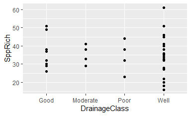
Does it make sense to arrange drainage classes in this way (i.e., alphabetically)? No.
ggplot(data = Oak, aes(x = DrainageClass.Ordered, y = SppRich)) + geom_point()
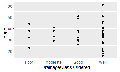
Note that the levels on the x-axis are now in order of increasing drainage.
If we were confident that we did not need the data in the original class any more, we could have overwritten it by assigning the results of this command to that object. However, ordinal factors are analyzed via polynomials rather than via ANOVA:
summary(lm(SppRich ~ DrainageClass, data = Oak))
summary(lm(SppRich ~ DrainageClass.Ordered, data = Oak))
I therefore find it helpful to keep both variables so that I can use the unordered factor for analysis and the ordered factor for graphing.
Indexing
One powerful feature of R is the ability to index objects to extract or manipulate elements that meet certain criteria. The type of indexing depends on the class of the object.
With one-dimensional objects (which classes?), indexing is done by using square brackets to reference the desired element(s) by their position in the sequence. For example, if we want the fourth element in y:
y[4]
With two-dimensional objects (which classes?), indexing requires two pieces of information to reference the rows and columns of the desired element(s). This can be done using square brackets to refer to the [row, column] of interest. If we want all row or all columns, we can leave that part of the indexing blank – while still including the comma. Here, we will create a simple data frame containing x, y, and z – all of which were created above – and then index it.
xyz <- data.frame(cbind(x, y, z))
xyz[ , 2] # all data from second column
xyz[ , "y"] # ditto
xyz[2 ,] # all data from second row
xyz[c(2:3), ] # data from second and third rows
xyz[-1, ] # all data except the first row
xyz[2 , 2] # data from second row, second column
xyz[2 , "y"] # ditto
For clarity, it is recommended to include a space after the comma within the brackets. Some folk leave a space before the comma too. These spaces do not affect the indexing.
Columns within a data frame can also be indexed by name using the string symbol ($):
xyz$x
Note that this column is a one-dimensional vector, so if we are calling it then further indexing of elements within it are the same as for other one-dimensional objects:
xyz$x[3]
Key Takeaways
Index a one-dimensional object via [item]. For example, the 2nd observation in the object x: x[2]
Index a two-dimensional object:
- Via
[row, column]. For example, the 2nd observation in the 1st row of column 1 in the objectxyz:xyz[2, 1] - If the object has named columns, use
$to return a column by name:object$column_name
When possible, index by name rather than by position.
Similarly, we can index our Oak data frame to focus on individual plots (rows) and/or variables (columns). Some examples:
Oak[ , 1] # Refers to all data from column 1 (plot elevation)
Oak[ , "Elev.m"] # Ditto
Oak$Elev.m # Ditto – but only works for data frame columns
Oak[1:2 , ] # Refers to all data from rows 1 and 2
Oak[c("Stand01","Stand02") , ] # Ditto
Oak[-5 , 1] # All elevations except that in the 5th row
What is the elevation of stand 02? ________________
Different types of indexing can be combined together. For example, we could choose particular columns to focus on and then index the rows of those columns. The next section presents three ways to conduct sequential actions on an object.
Conducting Multiple Sequential Actions
Often we want to conduct multiple actions in a sequence. For example, we might want to index a subset of the data that meets particular conditions. This can be done in at least three ways: as a series of separate actions, nested functions, and piping. I’ll illustrate these using an example in which we want to calculate how many plots have an elevation above 100 m.
A Series of Separate Actions
The easiest way to solve this example is with a series of steps. Here’s one solution:
oak_elevations <- Oak$Elev.m

gt100 <- oak_elevations > 100
sum(gt100)
[1] 35The first step indexed the column of interest. The second step evaluated whether each value met the criterion – the resulting object, gt100, consists of a series of trues and falses. TRUE is automatically treated as 1 and FALSE as 0, so in the third step we summed them to produce the answer.
The disadvantage of this approach is that we’ve created intermediate objects (oak_elevations, gt100) for which we have no other use. Intermediate objects like this can be cumbersome if they are not also needed later in the code, and can make it difficult to keep track of the objects that we do want to use later. If there are small numbers of them, they can be manually removed:
rm(oak_elevations, gt100)
Nested Functions
By nesting one function inside another, we could have done all of these actions in a single step:
sum(Oak$Elev.m > 100)
[1] 35Nested functions are common and very useful. However, they can be complicated to write, particularly because each function may have associated arguments that need to be referenced within the set of parentheses relating to that function – and it can be confusing to keep track of all those parentheses. For example, here is a more complicated example in which we index some data, relativize it, and then calculate the Euclidean distance between every pair of samples. We’ll learn soon what relativizing means and what a Euclidean distance is, but for now just observe how I’ve written this code with indenting and colors to illustrate the nested functions and show the function to which each argument belongs:
library(vegan)

geog.dis <- vegdist(
x = decostand(
x = Oak[,c("LatAppx","LongAppx")],
method = "range"),
method = "euc")
Here is the same code in a compact form (i.e., without indenting or named arguments):
geog.dis <- vegdist(decostand(Oak[,c("LatAppx","LongAppx")], "range"), "euc")
Nested functions have several disadvantages:
- It can be confusing to keep track of which set of parentheses relates to which function.
- Interpreting code can be challenging: you have to start from the inner-most set of parentheses and work your way outward (in both directions!).
- Adjusting code can be challenging. In particular, if we want to remove an intermediate step in a series of nested functions, we need to determine which parentheses and arguments to remove. Imagine removing
decostand()from the above code.
Piping
The pipe is an operator that allows you to feed the output of one function directly into another function. It is a technique that I find extremely helpful. See chapter 14 of Wickham & Grolemund (2017) for more information and examples of piping.
Piping is available through the pipe operator, %>%, in the magrittr package. Beginning in version 4.1.0, the ‘forward pipe’ (|>) is included in the base functionality of R. From what I have observed so far, these operators function identically.
The pipe is used at the end of one line to indicate that the output of that line is input for the next line. Specifically, the output of one line is input for the first argument of the function on the next line. Wickham & Grolemund (2017) describe it as focusing on verbs (actions), rather than nouns.
Applying similar actions to our data:
Oak |>
  filter(Elev.m > 100) |>

pull(Elev.m) |>
length()
[1] 35This may look more complicated than necessary for a simple example, but piping can be powerfully applied to more complicated sets of functions. For example, here is the more complicated example as in the nested functions above, and with the same color-coding:
library(magrittr)
geog.dis <- Oak[,c("LatAppx","LongAppx")] |>
decostand("range") |>
vegdist("euc")
Note how much easier this is to read than a set of nested functions. The steps are listed in the order they are implemented, rather than having to read outward from the inner-most function. This makes the code easier to write and to tweak. For example, if I wanted to exclude one step from the set of functions, I can simply comment out that line.
One caveat is that not all functions work within pipes (this is why I didn’t use the same functions to calculate the number of stands with elevations above 100 m), although I expect that to change now that piping is built into the base R installation – existing functions will be increasingly updated to work with the |> function.
Key Takeaways
Piping allows code to be easily read – steps are listed in the order they are implemented – and modified.
The %>% and |> operators are largely interchangeable.
When viewing code that includes a pipe, think of it as the phrase “and then”. For example, this code takes the object Oak and then filters it to those observations with elevation above 100 m:
Oak |> filter(Elev.m > 100)
Descriptive Statistics
Without indexing, functions are automatically applied to all columns in a matrix or data frame. This is evident if you use the summary() and str() functions:
summary(Oak)
str(Oak)
Note that different types of data are summarized as appropriate, and that the class of each column is identified in its structure. Functions can be applied to rows within the apply() function.
Once we know how to index our data, we can apply functions to the selected elements:
summary(Oak[ , 1]) # Returns range, mean, and quantiles

summary(Oak[ , "Elev.m"]) #equivalent - range, mean, and quantiles
stem(Oak[ , 1]) # Stem and leaf plot
hist(Oak[ , 1]) # Histogram
There are many other standard functions that can be used to examine your data: max(), min(), quantile(), range(), etc. You can also create your own functions – we’ll explore this later.
Borcard et al. (2018) note the importance of exploratory data analysis – visualizations and simple statistics – when familiarizing yourself with a dataset. They illustrate how the above functions, and many others, can be used to do so. Zuur et al. (2010) also provide helpful ideas about exploratory data analysis.
Manipulating Data in R
The Tidyverse
 Data can be manipulated using base R functions, but more intuitive means of doing so have been developed. In particular, Hadley Wickham and colleagues have produced the tidyverse, a number of ‘opinionated’ packages that share the same grammar. Key aspects include:
- Ability to pipe
- Don’t need to put column names in quotation marks (usually) when calling them
- Consistent terminology that works across packages
These packages can be installed en masse by installing the tidyverse package. It includes the following core packages:
readr, for data importtibble, for a modern re-imagining of data framesdplyr, for data manipulationtidyr, for data tidyingpurrr, for functional programmingggplot2, for data visualizationstringr, for working with strings (characters)forcats, for working with factorslubridate, for working with dates and times
These packages are the focus of the book by Wickham & Grolemund (2017) and its associated website (or the second edition of this book, which has its own website). And, links to cheatsheets for most of these packages have also been provided above. One way to consider how these packages interrelate is as follows:

Some additional packages are also available with more specialized applications – see the tidyverse website for details. In particular, I would highlight:
readxl, for reading Microsoft Excel spreadsheetsgoogledrive, for interacting with files stored on Google Drivemagrittr, for the pipe (%>%). Note that this has been incorporated into the base functionality of new versions of R as|>and is being replaced by it.tidymodels, for modeling and machine learning. This is actually a collection of packages, like the coretidyverse. Most are for parametric models; I haven’t investigated their application with the types of models that we focus on in this course.broom, for organizing model output
As an example of the tidyverse grammar, let’s work with the stand-level attributes related to soil groups and soil series. Let’s find out how many stands occur in each combination of soil group and soil series, and calculate summary statistics about species richness in each combination. We’ll use piping so that the output of one function is the input of the next function.
Oak.soil.sum <- Oak %>%
group_by(SoilGroupName, SoilSeriesName) %>%
summarize(N = length(SppRich),
MinS = min(SppRich),
MeanS = round(mean(SppRich), 1),
MaxS = max(SppRich),
.groups = "keep")
Oak.soil.sum
# A tibble: 7 × 6
# Groups:   SoilGroupName, SoilSeriesName [7]
  SoilGroupName SoilSeriesName     N  MinS MeanS  MaxS
  <chr>         <chr>          <int> <int> <dbl> <int>
1 Alluvial      Amity              3    32  38      44
2 Basic.igneous Dixonville         5    27  38.4    61
3 Basic.igneous Nekia              4    32  39      51
4 Basic.igneous Olympia            2    28  31      34
5 Sedimentary   Carlton            6    23  29.2    35
6 Sedimentary   Peavine            5    33  37.4    41
7 Sedimentary   Steiwer           22    16  33.3    51
Note that we created, and named, new variables for the number of stands (N) in each group along with the minimum, average, and maximum species richness in each group.
This type of summary is helpful both when manipulating data and when summarizing it for graphing purposes, etc.
plyr
The plyr package is related to the tidyverse (but not included in it), and is one I’ve found particularly helpful. The basic process within plyr is to split an object, do something to it, and then re-combine it (Wickham 2011).
There are several functions within plyr that have the same structure and naming convention:
- The first letter (a, d, or l) indicates whether it starts with an array, data frame, or list
- The second letter (also a, d, or l) indicates whether it produces an array, data frame, or list.
For example, ddply() takes a data frame, does something to it, and produces a new data frame. Its usage is:
ddply(.data, .variables, .fun = NULL, ..., .progress = "none", .inform = FALSE, .drop = TRUE, .parallel = FALSE, .paropts = NULL)
The key arguments are:
.data– the data frame to be processed.variables– the variables to use when splitting the data frame.fun– the function to apply to each piece after splitting
New variables can be created and named as part of this process.
This package uses the period function (.()) to allow column names to be specified without having to place them in quotation marks.
As an example, let’s do the same calculation of species richness in each combination of soil group and soil series:
library(plyr)
Oak.soil.sum <- ddply(.data = Oak,
.variables = .(SoilGroupName, SoilSeriesName),
.fun = summarize,
N = length(SppRich),
MinS = min(SppRich),
MeanS = round(mean(SppRich), 1),
MaxS = max(SppRich))
Oak.soil.sum
  SoilGroupName SoilSeriesName  N MinS MeanS MaxS
1      Alluvial          Amity  3   32  38.0   44
2 Basic.igneous     Dixonville  5   27  38.4   61
3 Basic.igneous          Nekia  4   32  39.0   51
4 Basic.igneous        Olympia  2   28  31.0   34
5   Sedimentary        Carlton  6   23  29.2   35
6   Sedimentary        Peavine  5   33  37.4   41
7   Sedimentary        Steiwer 22   16  33.3   51
This object is identical to that produced via piping, except that it is saved as an object of class ‘data.frame’ instead of class ‘tibble’.
Of course, this like all other code can be streamlined by omitting the argument names if the arguments are called in order:
Oak.soil.sum <- ddply(Oak, .(SoilGroupName, SoilSeriesName), summarize,
N = length(SppRich),
MinS = min(SppRich),
MeanS = round(mean(SppRich), 1),
MaxS = max(SppRich))
Oak.soil.sum
merge()
An essential function to be familiar with when you want to combine objects is merge(), which allows you to combine two objects on the basis of one or more specified columns. This is a base R function. Its usage is:
merge(x, y, by = intersect(names(x), names(y)), by.x = by, by.y = by, all = FALSE, all.x = all, all.y = all, sort = TRUE, suffixes = c(".x",".y"), no.dups = TRUE, incomparables = NULL, ...)
The key arguments are:
x,y– the data frames to be combined. Note that if you want to only include certain columns from a data frame you can index them here. Be sure, however, that you index it to include both the column(s) that form the basis for merging (needed for thebyargument) and the column(s) that you want to include in the resulting object.by,by.x,by.y– the columns to use as the basis for merging. If the columns have the same name, you can use thebyargument. If the column names differ between objects, specify the relevant columns viaby.xandby.y. Merging can also be done on the basis of row names by setting any of these equal to"row.names".all,all.x,all.y– whether to include rows that do not have a match in the other object. As for thebyargument, theallargument keeps all rows from both objects whileall.xonly keeps those fromxandall.yonly keeps those fromy. The default (all = FALSE) is to keep only those rows that are present in both objects.suffixes– text to append to the end of column names when column(s) with the same name occur in both data frames but are not part of the criteria for merging. Sometimes it is helpful to change the defaults so that column names from one data frame are unchanged after merging and thus still work with your previous code. For example, to keep column names fromxunchanged while distinguishing those fromy, we could setsuffixes = c("",".y").
As an example, let’s associate the mean species richness values for each soil group and soil series (calculated above) with the individual observations:
Oak$Stand <- row.names(Oak)
Oak.new <- merge(
x = Oak[ , c("SoilGroupName", "SoilSeriesName", "Stand", "SppRich") ],
by = c("SoilGroupName", "SoilSeriesName"),
all = TRUE,
y = Oak.soil.sum[ , c("SoilGroupName", "SoilSeriesName", "MeanS") ] )
Some notes about this code:
- I indexed
xandyto only include the variables being used for merging and the variables that I wanted to keep in the new object (Oak.new). If I did not do this, then all of the columns from both objects would have been retained. - I was able to use the
byargument (rather thanby.xandby.y) because the columns forming the basis of the merge had the same name in both objects. - When these objects do not contain the exact same set of observations, the
allargument and its variations are important. In this case, every observation was present in both objects.
Viewing the first few rows of output:
head(Oak.new)
  SoilGroupName SoilSeriesName   Stand SppRich MeanS
1      Alluvial          Amity Stand01      32  38.0
2      Alluvial          Amity Stand46      38  38.0
3      Alluvial          Amity Stand44      44  38.0
4 Basic.igneous     Dixonville Stand42      33  38.4
5 Basic.igneous     Dixonville Stand41      38  38.4
6 Basic.igneous     Dixonville Stand12      33  38.4
One very helpful way to diagnose functions like this is to keep track of the dimensionality of the starting and ending objects. Here, we began with a 47 x 4 object (four columns from Oak) and a 7 x 3 object (3 columns from Oak.soil.sum), and ended with a 47 x 5 object – the number of columns increased by one because we used two columns to index the two objects and added a single column of data. The number of rows didn’t change because every observation from Oak matched an observation from Oak.soil.sum.
Merging can also be applied within piping – the value that is fed into merge() is assumed to belong to the first argument (x). I’ll illustrate this by doing the same calculations as above while also using some additional tidyverse functions:
Oak.new <- Oak %>%
mutate(Stand = row.names(Oak)) %>%
  dplyr::select(SoilGroupName, SoilSeriesName, Stand, SppRich) %>%

merge(by = c("SoilGroupName", "SoilSeriesName"),

all = TRUE,

y = Oak.soil.sum[ , c("SoilGroupName", "SoilSeriesName", "MeanS") ])
Verify that the resulting object is the same.
The dplyr package also includes a family of functions to join (merge) objects:
inner_join(x, y): only include observations that match in bothxandy.left_join(x, y): include all observations ofxregardless of whether they matchy.xis assumed to be your primary table, so this is the most commonly used join. If a row doesn’t match, the new variables are filled in with missing values.right_join(x, y): include all observations ofyregardless of whether they matchx. If a row doesn’t match, the new variables are filled in with missing values.full_join(x, y): include all observations ofxand ofy. If a row doesn’t match, the new variables are filled in with missing values.
More information on these and other “two-table verbs” is available at https://dplyr.tidyverse.org/articles/two-table.html.
Conclusions
Understanding how to name and manipulate objects in R is foundational for all other aspects of this course. Much of the debugging that inevitably occurs during coding relates to how data are being manipulated.
References
Adler, J. 2010. R in a nutshell: a desktop quick reference. O’Reilly, Sebastopol, CA.
Borcard, D., F. Gillet, and P. Legendre. 2018. Numerical ecology with R. 2nd edition. Springer, New York, NY.
Çetinkaya-Rundel, M. 2023. Teaching the tidyverse in 2023. https://www.tidyverse.org/blog/2023/08/teach-tidyverse-23/
Crawley, M.J. 2012. The R book. Second edition (First edition, 2007). Wiley, West Sussex, England.
Dalgaard, P. 2008. Introductory statistics with R. Second edition (First edition, 2002). Springer, New York, NY.
Filazzola, A., and C.J. Lortie. 2022. A call for clean code to effectively communicate science. Methods in Ecology and Evolution 13:2119-2128.
Manly, B.F.J., and J.A. Navarro Alberto. 2017. Multivariate statistical methods: a primer. Fourth edition. CRC Press, Boca Raton, FL.
Paradis, E. 2005. R for beginners. Université Montpellier II, Montpellier, France. http://cran.r-project.org/doc/contrib/Paradis-rdebuts_en.pdf
Robinson, A. 2016. icebreakeR. https://cran.rstudio.com/doc/contrib/Robinson-icebreaker.pdf
Sellors, M. 2019. Field guide to the R ecosystem. http://fg2re.sellorm.com/
Torfs, P., and C. Brauer. 2014. A (very) short introduction to R. http://cran.r-project.org/doc/contrib/Torfs+Brauer-Short-R-Intro.pdf
Venables, W.N, D.M. Smith, and the R Development Core Team. 2023. An introduction to R. Version 4.3.2. http://cran.r-project.org/doc/manuals/R-intro.pdf
Wickham, H. 2011. The split-apply-combine strategy for data analysis. Journal of Statistical Software 40:1-29. http://www.jstatsoft.org/v40/i01/.
Wickham, H. 2014. Advanced R. Chapman & Hall/CRC, Boca Raton, FL.
Wickham, H. 2020. The tidyverse style guide. https://style.tidyverse.org/
Wickham, H., and G. Grolemund. 2017. R for data science: import, tidy, transform, visualize, and model data. O’Reilly, Sebastopol, CA. http://r4ds.had.co.nz/
Zuur, A.F., E.N. Ieno, and C.S. Elphick. 2010. A protocol for data exploration to avoid common statistical problems. Methods in Ecology and Evolution 1:3-14.
Media Attributions
- drainage.unordered
- drainage.ordered
- tidyverse
- tidyverse_packages © Çetinkaya-Rundel
