Introduction

SIMPER and Indicator Species Analysis can compare species patterns among categorical groups.  However, what if you want to relate species abundances to continuously distributed variables such as light availability or elevation or heat load?  That’s where TITAN (Threshold Indicator Taxa ANalysis) comes in.

TITAN

TITAN (Threshold Indicator Taxa ANalysis) was proposed by Baker & King (2010, 2013; King & Baker 2010).  The following figure provides a helpful, though detailed. flowchart of the process.

TITAN is a blend of univariate regression trees and ISA:

• Like a regression tree, TITAN considers all possible values that split the environmental variable into two groups:
  • The set of low values (z-).  The species in this group respond negatively to increases in the environmental gradient, and therefore are also called decreasers.
  • The set of high values (z+).  The species in this group respond positively to increases in the environmental gradient, and therefore are also called increasers.
• For each split of the environmental variable, TITAN conducts an ISA.  This summarizes, for each species, whether it is more strongly associated with z- or z+ and the value of the Indicator Value (IndVal).

After testing all possible values, each species is assigned to the group in which it produced the highest IndVal (step 2.1 in above figure).  The values of the environmental gradient are then permuted and IndVal is recalculated (step 2.2 in above figure).  These permutations are used to standardize the observed IndVals as z scores.  The value of the environmental variable that produced the strongest separation into two groups is called the change point.  In other words, this is the value of the environmental gradient that most strongly separated this taxon into two groups such that it was as strong as possible of an indicator for one of the two groups.

If we focused only on the observed data, we would not be able to assess statistical significance.  To do so, TITAN uses bootstrap resampling (step 4 in above figure).  This is a permutation-based procedure that we referenced a few weeks ago in the context of random forests.  If the abundance of a species is not related to the environmental variable, this could be evident in two ways:

• Species would be assigned to the z- group in some permutations and to the z+ group in other permutations.
• The species would not be a strong indicator of the group to which it was assigned.

Two metrics are used to evaluate the strength of the relationship as determined through the bootstrap resampling (step 5 in above figure):

• Purity: is the species response consistently assigned in the same direction?  In other words, is the species consistently assigned to either the z- or z+ group?
• Reliability: is the species a strong indicator of the group to which it is assigned?  In other words, in how many of the bootstrap permutations is IndVal determined to be statistically significant?

TITAN’s computations take more time than any of the other techniques that we’ve covered, because each species is tested individually against each potential split within the continuous variable, with bootstrapping to estimate uncertainty.

Finally, TITAN allows for the evaluation of individual species and of the community as a whole.

Published TITAN Examples

At UW’s Pack Forest, McBurney et al. (2017) examined the ectomycorrhizal fungal (EMF) community of a red alder stand and used TITAN to relate the abundance of these species to several environmental variables.  For example, some EMF taxa were more common at low soil moisture values and others were more common at high soil moisture values.

Smucker et al. (2020) showed that diatom OTUs relate to nutrient concentrations in streams, while Beauchene et al. (2014) related summer stream temperatures to the abundances of various fish taxa.

Martin & Hamman (2016) used TITAN to relate plant life forms to fire severity.

Morissette et al. (2019) identified a suite of bird species that responded positively to conversion of boreal forest to agriculture and a separate suite of birds that responded negatively to this conversion.  Similarly, Farwell et al. (2020) identified threshold amounts of forest loss affecting songbirds.

Costas et al. (2018) related the abundances of macroinvertebrate taxa to heavy metal levels in sediments.

TITAN in R (TITAN2::titan())

TITAN is available in R through the TITAN2 package.  Baker et al. (2020) provide a useful tutorial to the package; I encourage you to work through their examples.

The titan() function is the primary wrapper function in this package.  Its usage is:

titan(env,
txa,
minSplt = 5,
numPerm = 250,
boot = TRUE,
nBoot = 500,
imax = FALSE,
ivTot = FALSE,
pur.cut = 0.95,
rel.cut = 0.95,
ncpus = 1,
memory = FALSE,
messaging = TRUE
)

The key arguments (noting that some are abbreviations that can be easily misspelled) are:

• env – the environmental gradient to be tested (i.e., a vector)
• txa – the compositional matrix
• minSplt – the minimum split size to use during partitioning.  Default is 5.  In other words, the smallest number of samples in z- or z+ will be 5; all other samples will be in the other group.
• numPerm – number of random permutations to be used during ISA – these are used to derive a distribution of IndVal values for each species.  Default is 250, but package authors recommend increasing this to 500 or 1000 during formal analyses so there is less variation among runs.  However, increasing this necessarily increases computation time.
• boot – whether to conduct bootstrap resampling (TRUE) or not (FALSE).  Default is to do so (and is strongly recommended by package authors).
• nBoot – number of replicates to use during bootstrap resampling.  Default is 500, but package authors recommend using 500 or 1000 for formal analyses.
• imax – whether to determine taxon-specific change points based on indicator value (IndVal) maxima (TRUE) or z-score maxima (FALSE; the default).
• ivTot – whether to calculate indicator value (IndVal) scores using total relative abundance (TRUE) or mean relative abundance (FALSE; the default).
• pur.cut – cut-off proportion for determining purity (pure response direction) across bootstrap replicates.  The default (0.95) means that 95% of the results from bootstrap replicates agree with the observed response direction.
• rel.cut – cut-off proportion for determining reliability (reliable response magnitude) across bootstrap replicates.  The default (0.95) means that 95% of the results from bootstrap replicates have an IndVal p-value < 0.05.

The resulting object is a list with several elements, including:

• sppmax – a table showing the summary statistics for each species:
  • ienv.cp – change point if based on IndVal maximum.  Ignore unless you set imax = TRUE.
  • zenv.cp – change point if based on z-score maximum (default setting)
  • freq – frequency; number of non-zero abundance values
  • maxgrp – in which group the species had its maximum IndVal.  Either 1 (z- group) or 2 (z+ group).
  • IndVal – the maximum IndVal statistic (range = 0-100%) for the species
  • obsiv.prob – Probability of an equal or larger IndVal from random permutations.  Used for calculation of reliability.
  • zscore – IndVal expressed as a z-score
  • 5%, 10%, 50%, 90%, 95% – change point quantiles among bootstrap replicates
  • purity – proportion of replicates for which maxgrp matches observed maxgrp
  • reliability – proportion of replicates with obsiv.prob ≤ 0.05
  • z.median – median z-score across replicates
  • filter – 0 if species did not meet purity and reliability criteria, otherwise 1 (z- group) or 2 (z+ group)
• sumz.cp – observed community-level (i.e., across species) change point (cp) and quantiles associated with its distribution as determined by resampling.  Values are summarized for:
  • All species associated with smaller values of the environmental variable (row ‘sumz-‘)
  • All species associated with higher values of the environmental variable (row ‘sumz+’)
  • Filtered values, using only those species that were pure and reliable indicators of the group defined by smaller values of the environmental variable (row ‘fsumz-‘).
  • Filtered values, using only those species that were pure and reliable indicators of the group defined by higher values of the environmental variable (row ‘fsumz+’).

If cp for either filtered group differed strongly from the corresponding cp based on all species (e.g., ‘fsumz-‘ vs. ‘sumz-‘), it would be an indication that impure or unreliable indicators were substantially affecting the scores.

Some examples of how these output can be explored tabularly and graphically are shown below.

Oak Example: Responses to PDIR

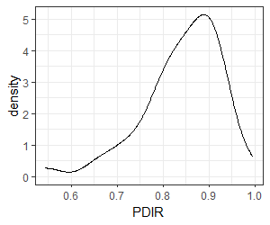
Let’s relate our oak compositional data to PDIR, the potential direct incident radiation (MJ/cm²/year).  The stands span a relatively wide range of PDIR values:

ggplot(data = Oak_explan, aes(x = PDIR)) +
geom_density() +
theme_bw()

Furthermore, we established in the beginning of this section that PDIR is significantly associated with differences in species composition:

set.seed(42)

adonis2(Oak1 ~ PDIR,
data = Oak_explan,
distance = "bray")

Permutation test for adonis under reduced model
Terms added sequentially (first to last)
Permutation: free
Number of permutations: 999

adonis2(formula = Oak1 ~ PDIR, data = Oak_explan, distance = "bray")
         Df SumOfSqs      R2      F Pr(>F)   
PDIR      1   0.8068 0.06958 3.3655  0.002 **
Residual 45  10.7881 0.93042                 
Total    46  11.5949 1.00000                 
---
Signif. codes:  
0 ‘***’ 0.001 ‘**’ 0.01 ‘*’ 0.05 ‘.’ 0.1 ‘ ’ 1

How do species relate to this environmental gradient?

set.seed(42)

titan.PDIR <- titan(env = Oak_explan$PDIR,
txa = Oak1)

Notes:

• We’ve accepted most defaults here
• The response and explanatory variable are reversed here from most (all?) other functions that we’ve seen
• This function will take a few minutes to run!

Individual Species Responses to PDIR

We’ll start by focusing on individual species responses.  We’ll limit our attention to the key columns, and only display the first few species here:

titan.PDIR$sppmax %>%
as.data.frame() %>%
select(zenv.cp, freq, maxgrp, IndVal, purity, reliability, filter) %>%
head()

         zenv.cp freq maxgrp IndVal purity reliability filter
Quga.t 0.7256032   47      1  54.19  0.534       0.660      0
Rhdi.s 0.8115082   47      2  59.67  0.624       0.812      0
Syal.s 0.9198630   46      1  93.51  0.988       0.980      1
Amal.s 0.9198630   41      1  81.56  0.466       0.910      0
GAL    0.9040936   41      1  59.70  0.580       0.578      0
Povu   0.9296631   41      1  57.53  0.542       0.684      0

For example, the light level that most strongly differentiates plots with and without Quga.t is zenv.cp = 0.7256.  Quga.t is more strongly associated with PDIR values below this value (maxgrp = 1).  In this group, it has an IV of 54.19.  However, it is not a particularly strong indicator of this condition as bootstrap samples did not consistently identify it as an indicator of the low light group (purity = 0.534) and it was only a significant indicator in two-thirds of bootstrap samples (reliability = 0.660).

The species that respond strongly and consistently (i.e., that meet the purity and reliability criteria) are flagged with values of 1 or 2 in the ‘filter’ column.  We can filter the results to just these species:

titan.PDIR$sppmax %>%
as.data.frame() %>%
select(zenv.cp, freq, maxgrp, IndVal, purity, reliability, filter) %>%
filter(filter != 0) %>%
arrange(maxgrp, zenv.cp)

         zenv.cp freq maxgrp IndVal purity reliability filter
Hodi.s 0.7256032   15      1  89.98  1.000       1.000      1
Rupa.s 0.8162860    8      1  35.22  1.000       0.954      1
Liap   0.8181559   20      1  61.53  0.992       0.960      1
Rhpu.t 0.8328414    6      1  33.33  0.996       0.968      1
Osce.s 0.8737474   23      1  59.07  1.000       0.978      1
Pomu   0.8785627   38      1  92.87  1.000       1.000      1
Cipa   0.8785627   10      1  35.71  0.998       0.960      1
Tegr   0.8972871   24      1  65.22  1.000       0.998      1
Syal.s 0.9198630   46      1  93.51  0.988       0.980      1
Hype   0.7998248   31      2  68.48  0.994       0.988      2
Crdo.s 0.8219381   22      2  56.98  0.994       0.976      2
Hola   0.8496857   23      2  60.55  0.998       0.988      2
Quga.s 0.8519232   39      2  84.34  1.000       1.000      2
CAR    0.8737474   15      2  52.48  1.000       0.996      2
Viam   0.9198630   24      2  84.81  1.000       0.998      2
Popr   0.9198630   22      2  94.29  0.998       0.986      2
Agte   0.9198630   22      2  75.34  0.998       0.976      2
Feru   0.9198630   15      2  64.77  0.982       0.952      2
Acmi   0.9198630   10      2  55.67  1.000       0.956      2

The filtered species are arranged by the group they are associated with (maxgrp) and then by their change point (zenv.cp).  In this case:

• Nine species were pure and reliable decreasers (maxgrp = 1) – the abundance of these species increased as PDIR declined.
• Ten species were pure and reliable increasers (maxgrp = 2) – the abundance of these species increased as PDIR increased.

We can also view the change point criteria for each species.  By default, this figure focuses only on taxa that meet the purity and reliability criteria:

plot_taxa_ridges(titan.PDIR,
xlabel = "PDIR")

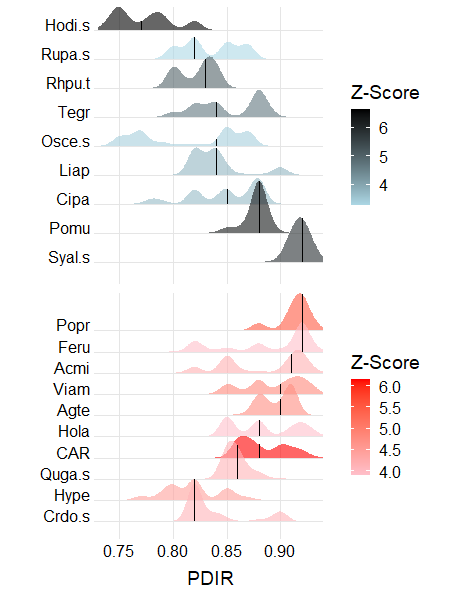
Species names are identified on the y-axis.  Species that are associated with smaller values (z-) or larger values (z+) of the environmental variable are shown separately and in different colors.  The intensity of the color relates to the strength of the z-score obtained for IndVal.  For each species, the change points show the probability density function of the bootstrapped replicates, and the vertical line is the median.

More detailed information about the change points identified through bootstrapping can be seen with the plot_cps() function:

plot_cps(titan.PDIR,
xlabel = "PDIR")

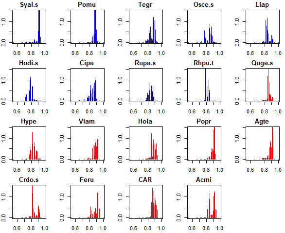
By default, this shows the change point distribution for each pure and reliable species.  As is the norm in this package, decreasers are shown in blue and increasers in red.  The distributions shown here are the same information that is shown in the ridge plot above.

A more interesting approach is to view the details for an individual species.  This is done by identifying the desired species with the taxaID argument.  (If you get an error about figure margins while running this line, clear all the plots from the plotting window first).

Let’s start by focusing on Hodi.s, the shrub that had the lowest change point in the ridge plot:

plot_cps(titan.PDIR,
taxaID = "Hodi.s",
xlabel = "PDIR")

In this graphic, the black open circles are the actual abundances of this species as a function of the PDIR of each sample unit.  The blue lines are the values of the change point identified in the bootstrap replicates.  The large open red circle is the value of the change point identified from the actual (observed) values.

Hodi.s was more likely to be encountered in shadier stands (PDIR < ~0.72) than in sunnier stands.

For comparison, here’s a graph for one of the increaser species:

plot_cps(titan.PDIR,
taxaID = "Popr",
xlabel = "PDIR")

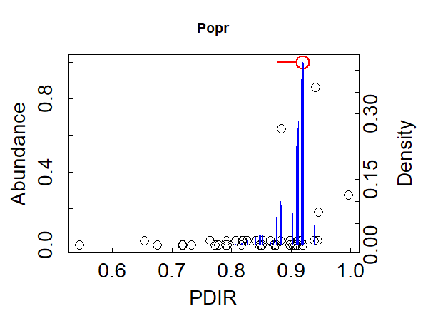
Although Popr usually had low relative abundance, it was more likely to be found at higher abundance in sunnier stands (PDIR values above 0.92).

(Note: Popr is an increaser in TITAN’s terminology and is shown in red when we view all species, but when viewing a single species the density distribution is shown in blue regardless of the group a species is associated with.)

Community-Level Change as a Function of PDIR

We’ve seen that TITAN distinguishes between species that are indicative of low values of the environmental gradient (z-; decreasers) and those that are indicative of high values of the environmental gradient (z+; increasers).  A community-level summary of how change relates to the environmental variable is accomplished by adding up the responses of the species in each group.  This can be done for all species (sumz- and sumz+ below) or for the filtered subset that meet the purity and reliability criteria (fsumz- and fsumz+ below).

The community-level summary is saved within the resulting object:

titan.PDIR$sumz %>%
round(3)

          cp  0.05  0.10  0.50  0.90  0.95
sumz-  0.833 0.726 0.748 0.817 0.852 0.876
sumz+  0.920 0.858 0.879 0.919 0.940 0.940
fsumz- 0.847 0.800 0.817 0.847 0.879 0.883
fsumz+ 0.920 0.849 0.851 0.879 0.920 0.939

The cp column reports the change points at which the community most strongly responded to the environmental variables.  In this case, species that respond negatively to PDIR (i.e., are shade tolerant) were most often at values below ~ 0.83 whereas those that respond positively to PDIR (i.e., are shade intolerant) were most often at values above 0.92.

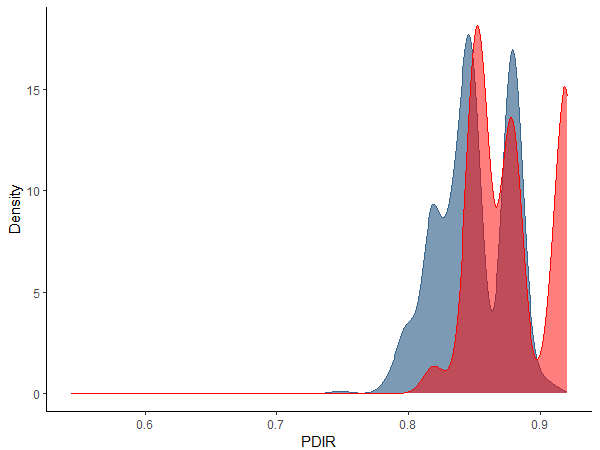
More details are evident graphically.  Here, I use the plot_sumz_density() function with a few arguments to customize the graphic – see the help file for information about these and other arguments.

plot_sumz_density(titan.PDIR,
ribbon = FALSE,
points = TRUE,
sumz = TRUE,
change_points = FALSE,
density = FALSE,
xlabel = "PDIR",
guide = "none")

This graph shows the magnitude of change for all taxa that strongly respond to PDIR (i.e., meet the purity and reliability criteria).  The horizontal axis is the range of values for PDIR – each unique value was measured in one or more stands.  The vertical axis is the sum of the z-scores of all species identified as pure and reliable indicators of either the z- group (decreasers; blue color) or the z+ group (increasers; red color).  Peaks indicate PDIR values at which there is lots of compositional change; plateaus indicate PDIR ranges in which there is little change in composition.

PS: The above graph focused on strong responders (i.e., species that met the purity and reliability criteria).  To see the community-level response based on all taxa, set filter = FALSE.  This looks quite different!

We can use that same function to view a different graphic:

plot_sumz_density(titan.PDIR,
ribbon = FALSE,
points = TRUE,
sumz = FALSE,
change_points = FALSE,
density = TRUE,
xlabel = "PDIR")

This graph shows the probability density of change points across the bootstrap replicates.  A narrow spread indicates a high degree of precision in the location of the community change point.  For example, this could occur if many species are responding similarly to the same value of the environmental gradient.  Usage of these density functions is left to the user – you could focus on the mode(s), for example, or the median.

Additional Applications of TITAN

In theory, many of the additional applications described for ISA can also be applied with TITAN.  For example, you could conduct non-hierarchical analyses and assess species that respond to either or both of two continuous variables.  Or, the outcome of a TITAN analysis of a continuous variable could be combined with the outcome of an ISA of a categorical variable.

The pTITAN2 package allows the user to identify environmental thresholds within a site and to test whether change points vary among sites.  For example, consider a site in which composition and an environmental variable such as PDIR are measured in a control area and in treated area.  This is a relatively new package; I have not yet seen it in use.

Recommendations for TITAN

Many of the recommendations for using ISA and combining the results of multiple sites or studies also apply to TITAN:

1. When collecting data, identify individuals to the finest taxonomic level possible.  Congeneric species, for example, may respond individually to environmental conditions.
2. Consider the proper exchangeable units for the permutations tests (Anderson & ter Braak 2003). TITAN does not allow the same level of control of permutations as is possible with ISA and many of the statistical techniques that we’ve discussed.
3. Direct comparisons of TITAN results from multiple studies would require that the continuous variables be measured in the same way in each study. Methods to do so should be described in detail.  However, these types of comparisons are going to be more challenging than for ISA. For example, the change point differs among species and would probably differ among studies for the same species – though I’m not aware of any examples that have done this to date.
4. Ensure that the sample size is sufficient to sample the vegetation and the environmental conditions.
5. Digital appendices and other repositories permit the archiving of data in an accessible manner (Parr & Cummings 2005).  Tracking species and the associated environmental variables requires more detailed data than is the case with the simplified ISA – the abundance of a species and the associated value of the environmental variable need to be recorded together as opposed to just knowing the abundance of the species and the group that each sample was part of.
6. To prevent publication bias in future meta-analyses (Gurevitch & Hedges 2001), publish data for all species, regardless of whether or not they were significant indicators.

Conclusions

TITAN is a computationally intensive amalgamation of techniques to explore how individual taxa relate to continuously-distributed variables.  These variables can be measured individually or they could be derived from a multivariate analysis of a larger set of environmental variables (e.g., Costas et al. 2018).

Data adjustments remain important; these calculations will be affected by adjustments.  Use the same adjustments as in all other aspects of your analysis.

References

Anderson, M.J., and C.J.F. ter Braak. 2003. Permutation tests for multi-factorial analysis of variance. Journal of Statistical Computation and Simulation 73:85-113.

Baker, M.E., and R.S. King. 2010. A new method for detecting and interpreting biodiversity and ecological community thresholds. Methods in Ecology and Evolution 1:25-37.

Baker, M.E. and R.S. King. 2013. Of TITAN and straw men: an appeal for greater understanding of community data. Freshwater Science 32:489-506.

Baker, M., R. King, and D. Kahle. 2020. An introduction to TITAN2. Version 2.4.3. https://cran.r-project.org/web/packages/TITAN2/vignettes/titan2-intro.pdf

Beauchene, M., M. Becker, C.J. Bellucci, N. Hagstrom, and Y. Kanno. 2014. Summer thermal thresholds of fish community transitions in Connecticut streams. North American Journal of Fisheries Management 34(1):119-131.

Costas, N., I. Pardo, L. Méndez-Fernández, M. Martínez-Madrid, and P. Rodríguez. 2018. Sensitivity of macroinvertebrate indicator taxa to metal gradients in mining areas in Northern Spain. Ecological Indicators 93:207-218.

Farwell, L.S., P.B. Wood, R. Dettmers, and M.C. Brittingham. 2020. Threshold responses of songbirds to forest loss and fragmentation across the Marcellus-Utica shale gas region of central Appalachia, USA. Landscape Ecology 35: 1353-1370.

Gurevitch, J., and L.V. Hedges. 2001. Meta-analysis: combining the results of independent experiments. Pages 347-369 in S.M. Scheiner and J. Gurevitch (editors). Design and analysis of ecological experiments. Oxford University Press, New York, NY.

King, R.S., and M.E. Baker. 2010. Considerations for analyzing ecological community thresholds in response to anthropogenic environmental gradients. Journal of the North American Benthological Society 29:998-1008.

Martin, R.A., and S.T. Hamman. 2016. Ignition patterns influence fire severity and plant communities in Pacific Northwest, USA, prairies. Fire Ecology 12:88-102.

McBurney, K.G., E.T. Cline, J.D. Bakker, and G.J. Ettl. 2017. Ectomycorrhizal community composition and structure of a mature red alder (Alnus rubra) stand. Fungal Ecology 27:47-58.

Morissette, J.L., E.M. Bayne, K.J. Kardynal, and K.A. Hobson. 2019. Regional variation in responses of wetland-associated bird communities to conversion of boreal forest to agriculture. Avian Conservation and Ecology 14(1):12.

Parr, C.S., and M.P. Cummings. 2005. Data sharing in ecology and evolution. Trends in Ecology and Evolution 20:362-363.

Smucker, N.J., E.M. Pilgrim, C.T. Nietch, J.A. Darling, and B.R. Johnson. 2020. DNA metabarcoding effectively quantifies diatom responses to nutrients in streams. Ecological Applications 30:e02205.