Theory

Permutational techniques do not assume homogeneity of variances.  However, patterns of dispersion (variability among sample units) can influence the interpretation of a statistical test.  Significant differences among groups may occur for either or both of two reasons (Warton et al. 2012):

• Differences in the means (centroids)
• Differences in the amount of dispersion of sample units around those centroids

These alternatives are nicely illustrated in two dimensions – see Figure 2.1 from Anderson et al. (2008), reproduced below.

Sensitivity to variability is not unique to multivariate analyses – groups in a univariate analysis can also differ with regard to their mean values, variation around those means, or both. In univariate analyses, dispersion can be examined using Levene’s test.  PERMDISP is a multivariate extension of Levene’s test (Anderson 2006) to examine whether groups differ in plot-to-plot variability.

In essence, PERMDISP involves calculating the distance from each data point to its group centroid and then testing whether those distances differ among the groups.  However, recall that distance measures such as Bray-Curtis are semi-metric … this means we cannot always calculate the centroid directly.  In practice, therefore, a Principal Coordinates Analysis (PCoA) is applied to the distance measure and the centroids are calculated on the basis of the coordinates in PCoA space.  See the ‘PCoA‘ chapter for more details on this technique.

Consider an example in which a PERMANOVA test has indicated a difference among groups.  Immediately, we know that the patterns are not as in Fig. 2.1a, but how do we determine whether the patterns are due to dispersion (Fig. 2.1c), location (Fig. 2.1b), or both (Fig. 2.1d)?  A non-significant result from PERMDISP would indicate that groups do not differ in dispersion and that therefore the differences are entirely due to differences in location (e.g., Fig. 2.1b).  A significant result from PERMDISP would indicate that the groups differ in dispersion.  However, it is not possible on the basis of these two tests to determine conclusively whether the groups differ only in dispersion (Fig. 2.1c) or both dispersion and location (Fig. 2.1d).  In research projects I’ve been involved with, we’ve visually explored our data to decide between these two options (this admittedly is not a very satisfying approach).

Anderson et al. (2008) include a chapter providing more detail about tests of homogeneity of dispersion.

Multivariate homogeneity – distance to group centroids – can also be used for other purposes:

• As a measure of beta diversity (Anderson et al. 2006)
• To estimate how the number of sampling units affects precision of compositional analyses (Anderson and Santana-Garcon 2015)

Anderson (2015) notes that dispersion is strongly affected by transformations applied to the original data and by the choice of distance measure.

If PERMDISP is being used as a follow-up to a PERMANOVA or other test, it is essential that the same data adjustments and distance measure be used in both cases, otherwise the tests are not directly comparable.

Basic Procedure

The basic procedure for PERMDISP is as follows:

1. Begin with a distance matrix.  Conduct a Principal Coordinates Analysis (PCoA) ordination of the distance matrix.  This expresses the sample units along new axes that are organized such that the first axis explains as much of the variation in the dataset as possible, the second axis explains as much of the remaining variation as possible, etc.
2. Overlay the grouping factor onto the PCoA.  In other words, code each sample unit based on the group to which it belongs.
3. Calculate the centroid (average score) for each level of the grouping factor in the ordination space.
4. Calculate the distance between each observation and the centroid of the group to which it belongs.

This technique differs from the others that we’ve covered as it does not involve a statistical test.  Rather, it produces a univariate dataset – the distance from each observation to the centroid of its group – that can be analyzed via other statistical tests.  This response is likely to be relatively normally distributed regardless of the characteristics of the multivariate data that formed the distance matrix, and therefore could be analyzed via techniques like ANOVA.  It of course could also be analyzed via PERMANOVA (vegan::adonis2()) or other permutation-based techniques.

Simple Example, Worked By Hand

I’ll illustrate this approach by working directly from the data rather than the distance matrix.  Our simple example is in Euclidean space so we can use techniques such as the Pythagorean formula to determine the group centroids.  I’m also going to skip the PCoA ordination that is described below – it rotates the dataset but doesn’t change the overall results when we work with Euclidean distances.

Begin by calculating the centroid for each group.

perm.eg.centroids <- perm.eg |>
group_by(Group) |>
summarize(Resp1.mean = mean(Resp1), Resp2.mean = mean(Resp2))

  Group Resp1.mean Resp2.mean
1 A              3        3  
2 B             10       10.3

Combine the raw data with the group means, and use Pythagorean theorem to calculate the distance from each observation to the mean of its group.

perm.eg <- perm.eg |>
merge(y = perm.eg.centroids) |>
mutate(distance = sqrt((Resp1 - Resp1.mean)^2 + (Resp2 - Resp2.mean)^2))

The column perm.eg$distance is the set of values that are produced by PERMDISP.

Implementation in R (vegan::betadisper())

Analyses of multivariate homogeneity of group dispersions (variances) can be done using the betadisper() function in the vegan package.  Its usage is:

betadisper(
d,
group,
type = c("median", "centroid"),
bias.adjust = FALSE,
sqrt.dist = FALSE,
add = FALSE
)

The main arguments are:

• d – distance matrix to be analyzed
• group – grouping factor
• type – type of analysis to perform: either adjust groups relative to their spatial median or to the group centroid.  The spatial median is the default though the centroid is commonly used.
• The other arguments here provide adjustments for small sample size, negative eigenvalues, etc.

This function conducts a PCoA of the distance matrix (to express semi-metric distances in Euclidean space), calculates the distance from each sample unit to the centroid for its level of the grouping factor, and saves these distances (and other things) in an object of class ‘betadisper’.  It does not test for differences in them.

Separate functions can be applied to an object of class ‘betadisper’ to accomplish different objectives:

• View data graphically
  • plot()
  • boxplot()
• Conduct statistical tests (note that these are univariate data!)
  • anova()
  • TukeyHSD()
  • permutest()

Simple Example

The bivariate response in our simple example differs between the two groups.  Do they differ in dispersion?

Use betadisper() to calculate the distance from each sample unit to the centroid of its group:

perm.eg.betadisper <- betadisper(d = dist(perm.eg[ , c("Resp1", "Resp2")]), group = perm.eg$Group, type = "centroid")

The data consist of the distance from each observation to the centroid of its group:

perm.eg.betadisper$distances

Confirm that these distances are identical to those that calculated by hand above.

We can graph the data:

plot(perm.eg.betadisper)

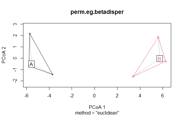
Key features to note in this plot:

• The ordination is the first two axes of the Principal Coordinates Analysis (PCoA).  With this bivariate dataset, the data cloud has simply been rotated so that the variation is aligned with the ordination axes.  The axes of the PCoA are combinations of the responses rather than individual responses.  The responses were combined in such a way that the first axis explains as much of the variation in the dataset as possible, and the second axis explains the remaining variation in this bivariate response.  We’ll talk about this more when we discuss ordinations.
• Plots are shown as points, with colors and shapes identifying the group to which they belong.
• A colored line outlines the perimeter or hull of the group in this ordination space.
• Each group is labelled at its centroid.
• A grey line connects each stand to its centroid. These lines are the distances that were calculated in betadisper().

We can whether the distances differ statistically:

anova(perm.eg.betadisper)

Of course, we could also do this as a permutation-based test.  Let’s use PERMANOVA to do so:

adonis2(dist(perm.eg.betadisper$distances) ~ perm.eg$Group)

This test is not significant, so there is no evidence of a difference in dispersion between the two groups.  This agrees with what we saw visually.

Grazing Example

We established previously that the composition of the oak plant community differs as a function of grazing history:

adonis2(Oak1.dist ~ grazing)

Permutation test for adonis under reduced model
Terms added sequentially (first to last)
Permutation: free
Number of permutations: 999

adonis2(formula = Oak1.dist ~ grazing)
         Df SumOfSqs      R2      F Pr(>F)    
grazing   1   0.6491 0.05598 2.6684  0.001 ***
Residual 45  10.9458 0.94402                  
Total    46  11.5949 1.00000                  
---
Signif. codes:  0 ‘***’ 0.001 ‘**’ 0.01 ‘*’ 0.05 ‘.’ 0.1 ‘ ’ 1

Let’s check whether these differences are due to location and/or dispersion.  Summarize dispersion relative to the group centroids:

graz.res.betadisper <- betadisper(d = Oak1.dist, group = grazing, type = "centroid")

The data consist of the distance from each observation to the centroid of its group:

graz.res.betadisper$distances

Our simple example was bivariate so it was easy to envision the centroids.  In this case the data are highly multivariate (based on 103 species).  The centroids, and the associated distance from each stand to its centroid, are calculated based on all axes.

To test for differences via ANOVA:

anova(graz.res.betadisper)

Analysis of Variance Table

Response: Distances
          Df   Sum Sq   Mean Sq F value Pr(>F)
Groups     1 0.000463 0.0004627  0.0974 0.7564
Residuals 45 0.213788 0.0047508 

The main effect of grazing is not significant, so there is no reason to test for pairwise differences between groups (and, we only have two groups anyways!).  However, we will do so anyways to show how it could be used in other analyses:

TukeyHSD(graz.res.betadisper)

  Tukey multiple comparisons of means
    95% family-wise confidence level

Fit: aov(formula = distances ~ group, data = df)

$group
              diff         lwr        upr     p adj
Yes-No -0.00653026 -0.04867375 0.03561323 0.7564127

If our grouping factor included three or more groups, there would be one line and test for each pair of groups.

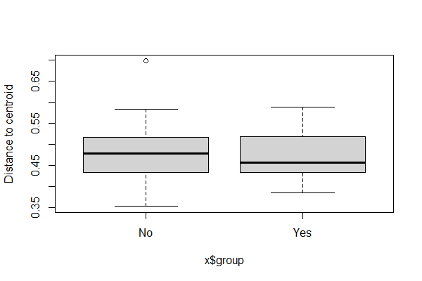
We conclude that, although composition differs among grazing statuses, it does so because of differences in location rather than dispersion.

Finally, let’s explore these distances visually.

When applied to an object of class ‘betadisper’, the boxplot() function creates a box-and-whisker plot showing the distance to the group centroid in each group.

boxplot(graz.res.betadisper)

And, as we’ve seen above, we can use the plot() function for an object of this class.

plot(graz.res.betadisper)

This plot is very similar to the one from the simple example but deserves a few additional comments:

• The underlying data are highly multivariate – 103 species – but we’re seeing just the first two axes of the Principal Coordinates Analysis (PCoA).  The procedure for calculating these axes means that each axis explains as much of the variation as possible that has not been explained by other axes.  In other words, there is no other two-dimensional representation of this dataset that reflects more of its variation than is possible with these two axes.
• A grey line connects each stand to its centroid in this 2-D ordination space. These lines are similar to but not exactly the same as the distances calculated in betadisper(), because the actual distances are based on the full PCoA (103 axes) rather than just the two axes shown here.

References

Anderson, M.J. 2006. Distance-based tests for homogeneity of multivariate dispersions. Biometrics 62(1):245–253.

Anderson, M.J. 2015. Workshop on multivariate analysis of complex experimental designs using the PERMANOVA+ add-on to PRIMER v7. PRIMER-E Ltd, Plymouth Marine Laboratory, Plymouth, UK.

Anderson, M.J., K.E. Ellingsen, and B.H. McArdle. 2006. Multivariate dispersion as a measure of beta diversity. Ecology Letters 9:683-693.

Anderson, M.J., R.N. Gorley, and K.R. Clarke. 2008. PERMANOVA+ for PRIMER: guide to software and statistical methods. PRIMER-E Ltd, Plymouth Marine Laboratory, Plymouth, UK. 214 p.

Anderson, M.J., and J. Santana-Garcon. 2015. Measures of precision for dissimilarity-based multivariate analysis of ecological communities. Ecology Letters 18(1):66-73.

Warton, D.I., S.T. Wright, and Y. Wang. 2012. Distance-based multivariate analyses confound location and dispersion effects. Methods in Ecology and Evolution 3:89-101.