Contents:

• Introduction
• ReDundancy Analysis (RDA)
• Distance-based ReDundancy Analysis (dbRDA)
• Oak Example
• Interpreting RDA and dbRDA
• Conclusions
• References

Introduction

Other than CCA, all of the ordination techniques that we’ve discussed thus far are unconstrained or indirect gradient analyses – the only information that is incorporated into the procedure is the matrix of response variables.  Constrained ordinations are direct gradient analyses.  These are analogous to regression, where the objective is to correlate the response matrix and one or more explanatory variables.

A 3-D conceptual example might help here.  Imagine the sample units as a point cloud.  We could view this point cloud from many different vantage points.  For example, we could view it from a spot where we see as much of the variation as possible – an unconstrained ordination is showing us the view from this spot.  Now imagine that the points are colored to reflect different groups.  Depending on where we view the point cloud from, these groups might appear more or less discrete.  A constrained ordination shows us the view from the spot where the groups are as distinct as possible.  These different perspectives are illustrated in the appendix.

In summary, different types of analyses provide different ways to view the point cloud:

• Unconstrained ordinations identify the perspective that shows as much of the variation in the point cloud as possible.
• Constrained ordinations view or interpret the point cloud from the perspective of the chosen explanatory variable(s).

We will consider two similar types of constrained ordinations, ReDundancy Analysis (RDA) and distance-based RDA (dbRDA).  Neither of these techniques is addressed by Manly & Navarro Alberto (2017).

ReDundancy Analysis (RDA)

Approach

Legendre & Legendre (2012; Section 11.1) describe ReDundancy Analysis (RDA) as “the direct extension of multiple regression to the modelling of multivariate response data” (p. 629).  It is based on Euclidean distances. Transformations and standardizations can be conducted at the user’s discretion outside of the analysis.

RDA uses two common techniques in sequence: “RDA is a multivariate (meaning multiresponse) multiple linear regression followed by a PCA of the matrix of fitted values” (Borcard et al. 2018, p. 205).

1. Regression: Each variable in the response matrix is fit to the variables in the explanatory matrix.  The regression model assumes that the explanatory and response variables are linearly related to one another.  This may require transformations.  The fitted values of each response variable with each explanatory variable are calculated.  The residuals (i.e., variation not accounted for by the explanatory variables) are also calculated – these are simply the original values minus the fitted values.

2. PCA: Two separate PCAs are conducted:
   1. A PCA on the matrix of fitted values. By conducting the PCA on the fitted values rather than the original values, the resulting eigenvalues and eigenvectors are constrained to be linear combinations of the explanatory variables.
   2. A PCA on the matrix of residuals.  These residuals are conditional: they are the variation that was not explained by the explanatory variables.

Notes:

• If no explanatory variables are provided, then the first step is meaningless: there are no fitted values, and the second step results in a regular PCA.
• The explanatory variables should not be highly correlated with one another. If two such variables are highly correlated, consider omitting one or using PCA first to reduce them to a single principal component.

The result of this process is a set of principal components conditioned (or weighted) by the explanatory variables.  “In RDA, one can truly say that the axes explain or model (in the statistical sense) the variation of the dependent [response] matrix” (Borcard et al. 2018, p. 205).

The degrees of freedom (df) required for the explanatory variables indicate how many axes are constrained by those variables.  For example, a single continuous variable requires 1 df, and a factor with m levels requires m-1 df.  The axes that are constrained by these variables are referred to as canonical axes or constrained axes.  As with a regular PCA, each of these axes is orthogonal to the others, and can be tested and evaluated individually.  Borcard et al. (2018) note that the eigenvalues associated with these axes measure the amount of variance explained by the RDA model.

Once the constrained axes have accounted for all of the variation that they can, the remaining variation is arrayed along unconstrained axes.  These are interpreted in the same way as in a PCA, except that they are explaining the variation that remains after having accounted for as much variation as possible through the constrained axes.  Borcard et al. (2018) note that the eigenvalues associated with these axes measure the amount of variance represented by these axes, but not explained by any included explanatory variable.

I have noted several times that PCs are always a declining function: the first explains as much variation as it can, the second as much as it can of the remaining, etc.  Constrained ordinations are a partial exception to this rule.  The constrained axes are a declining function and the unconstrained axes are also a declining function, but the transition from the last constrained axis to the first unconstrained axis may be associated with a (sometimes dramatic) increase in the magnitude of the eigenvalue.

RDA in R (vegan::rda())

In R, RDA can be conducted using function rda() in vegan.  Its usage is:

rda(formula,
data,
scale = FALSE,
na.action = na.fail,
subset = NULL,
...
)

The arguments are:

• formula – model formula, with the community data matrix on the left hand side and the explanatory (constraining) variables on the right hand side. Additional explanatory variables can be included that ‘condition’ the response – their effect is removed before testing the constraining variables.  See the help files for details of how to include conditioning variables.  The explanatory and response variables can also be specified as separate arguments, but the formula approach is preferred as it allows you to easily control which variables are being used.
• data – the data frame containing the explanatory variables.
• scale – whether to scale species (i.e., columns in the response matrix) to a variance of 1 (like a correlation). Default is to not do so (FALSE).  While this may make sense with other types of responses, Borcard et al. (2018) state that this should not be used with community data.
• na.action – what to do if there are missing values in the explanatory variables. Several options:
  • na.fail – stop analysis. The default.
  • na.omit – drop rows with missing values and then proceed with analysis.
  • na.exclude – keep all observations but return NA for values that cannot be calculated.
• subset – whether to subset the data, and how to do so.

The resulting object contains lots of different elements.  An object of class ‘rda’ can be subject to pre-defined methods for plot(), print(), and summary().

We have talked repeatedly about how it is more appropriate to summarize community composition data using Bray-Curtis rather than Euclidean distances.  I therefore will not illustrate RDA using our oak plant community dataset but will instead illustrate dbRDA below.

distance-based ReDundancy Analysis (dbRDA)

Approach

ReDundancy Analysis (RDA) is a constrained ordination that uses Euclidean distances.  Distance-based ReDundancy Analysis (dbRDA or db-RDA; Legendre & Anderson 1999) is a more general way to do the same type of constrained ordination; the generality arises because it can be applied to any distance or dissimilarity matrix.

The connection between RDA and dbRDA is simply the step of expressing a non-Euclidean dissimilarity matrix in a Euclidean space.  Sound familiar?  That’s what a PCoA does.

As a result, the first step of a dbRDA is to apply a PCoA to the distance matrix and to keep all principal coordinates.  As discussed in that chapter, this can be done regardless of the distance measure used (hence the generality of this technique).  By keeping all of the principal coordinates we have rotated the distance matrix and expressed it in Euclidean distances without reducing its dimensionality.

The second step of a dbRDA is to conduct a RDA on the principal coordinates.  In other words, the principal coordinates are subject to a multivariate multiple linear regression and then the fitted values and residuals are subject to separate PCAs.  This procedure maximizes the fit between the distance matrix containing the PCoA coordinates and the explanatory variables or constraints.

Notes:

1. If applied to a Euclidean distance matrix, dbRDA is identical to RDA.
2. If no explanatory variables are provided, a dbRDA is identical to a PCoA (because the first step results in a regular PCoA and the second step is meaningless).
3. Canonical Analysis of Principal coordinates (CAP) is another technique that has been proposed (McArdle & Anderson 2001; Anderson & Willis 2003). According to Borcard et al. (2018), it analyzes the dissimilarity matrix directly and does not require the initial PCoA. However, the help file for vegan::capscale() indicates that it is similar to dbRDA, and it appears that it is not maintained as a separate function.

db-RDA in R (vegan::dbrda() and vegan::capscale())

The help file describes these functions as ‘alternative implementations of dbRDA’.  These functions differ somewhat in their approach – including how they deal with and report on negative eigenvalues – but generally should give very similar results; see the help file for details.  Both are wrapper functions that call on other functions for various steps in the analysis.

The usage of dbrda() is:

dbrda(formula,
data,
distance = "euclidean",
sqrt.dist = FALSE,
add = FALSE,
dfun = vegdist,
metaMDSdist = FALSE,
na.action = na.fail,
subset = NULL,
...
)

The key arguments are:

• formula – model formula, with a community data frame or distance matrix on the left hand side and the explanatory (constraining) variables on the right hand side. Additional explanatory variables can be included that condition the response – their effect is removed before testing the constraining variables.  The explanatory and response variables can also be specified as separate arguments, but the formula approach is preferred as it allows you to easily control which variables are being used.
• data – the data frame containing the explanatory variables.
• distance – type of distance matrix to be calculated if the response is a data frame. Default is to use Euclidean distance.
• sqrt.dist – whether to transform the distance matrix by taking the square root of all dissimilarities. This can be helpful to ‘euclidify’ some distance measures.  Default is to not do so (FALSE).
• add – when conducting the PCoA, whether to add a constant to the dissimiliarities so that none of them are non-negative. Same options as for wcmdscale():  FALSE or TRUE or "lingoes" or "cailliez".  However, the default here is to not add a constant (FALSE) or, in other words, to permit negative eigenvalues in the results.  Setting this to TRUE is the same as add = "lingoes".
• dfun – name of function used to calculate distance matrix. Default is vegdist (i.e., vegdist()).
• metaMDSdist – whether to use the same initial steps as in metaMDS() (auto-transformation, stepacross for extended dissimilarities). Default is to not do so (FALSE).
• na.action – what to do if there are missing values in the constraints (explanatory variables). Same options as for wcmdscale().  Default is to stop (na.fail); other options are to drop sample units with missing values (na.omit or na.exclude).
• subset – whether to subset the data, and how to do so.

The resulting object contains lots of different elements.  Objects of class ‘dbrda’ or ‘capscale’ can be subject to pre-defined methods for plot(), print(), and summary().  By default, only the first 6 axes are reported – since the objective is to view patterns related to one or more explanatory variables, the user is unlikely to need or use other axes.

The function capscale() has extremely similar usage – see the help file for details.

Oak Example

Let’s use dbRDA to test the relationship between oak plant community composition and geographic variables.

source("scripts/load.oak.data.R")

geog.stand <- Oak %>%
select(c(LatAppx, LongAppx, Elev.m)) %>%
decostand("range")

Oak1_dbrda <- dbrda(Oak1 ~ Elev.m + LatAppx + LongAppx,
data = geog.stand,
distance = "bray")

print(Oak1_dbrda)

Call: dbrda(formula = Oak1 ~ Elev.m + LatAppx + LongAppx, data =
geog.stand, distance = "bray")

               Inertia Proportion Rank RealDims
Total         11.59490    1.00000              
Constrained    0.97790    0.08434    3        3
Unconstrained 10.61700    0.91566   43       33
Inertia is squared Bray distance 

Eigenvalues for constrained axes:
dbRDA1 dbRDA2 dbRDA3 
0.4568 0.3043 0.2168 

Eigenvalues for unconstrained axes:
  MDS1   MDS2   MDS3   MDS4   MDS5   MDS6   MDS7   MDS8 
1.7901 1.1519 1.0933 0.7744 0.7069 0.6514 0.5212 0.4344 
(Showing 8 of 43 unconstrained eigenvalues)

Much more extensive results is available through summary() and can be viewed in the Console or saved to an object:

Oak1_dbrda_summary <- summary(Oak1_dbrda)

Saving this output to an object allows its components to be explored and used for other purposes.

Interpreting the Output

Near the top of the output is a table showing of how the variance has been partitioned, which I’ve repeated here:

               Inertia Proportion Rank RealDims
Total         11.59490    1.00000              
Constrained    0.97790    0.08434    3        3
Unconstrained 10.61700    0.91566   43       33

In this case, 8.43% of the variance is accounted for by the constraining variables, the set of geographic variables.  The other 91.57% of the variance is unconstrained – it cannot be explained by the spatial location of the sample units.

Constrained Axes

The summary() output includes a summary of the constrained eigenvalues:

Oak1_dbrda_summary$concont

$importance
Importance of components:
                      dbRDA1 dbRDA2 dbRDA3
Eigenvalue            0.4568 0.3043 0.2168
Proportion Explained  0.4671 0.3112 0.2217
Cumulative Proportion 0.4671 0.7783 1.0000

As with other eigenvalues, these are a declining function: the first always accounts for the most variation, the second for the second-most variation, etc.  However, note that the proportion explained here is not the overall importance of each axis relative to the full variance in the dataset.  Rather, it is the proportion of the variance explained by these explanatory variables.  For example, dbRDA1 explains 46.71% of the 8.43% of the variance accounted for by these three variables.  Multiplying those two values together yields 3.94%, which is the amount of variance explained by dbRDA1 overall.

The relative importance of axes can be viewed.  By default, the first 6 dimensions are shown, even though only the first three axes are constrained in this example:

Oak1_dbrda_summary$cont

$importance
Importance of components:
                       dbRDA1  dbRDA2 dbRDA3   MDS1    MDS2    MDS3
Eigenvalue            0.45675 0.30432 0.2168 1.7901 1.15188 1.09331
Proportion Explained  0.03939 0.02625 0.0187 0.1544 0.09934 0.09429
Cumulative Proportion      NA      NA     NA     NA      NA      NA

Since we included three explanatory variables, the first three axes (dbRDA1, dbRDA2, dbRDA3) are constrained to maximize the correlation between the response matrix and the geographic explanatory variables.  These axes are, “in successive order, a series of linear combination of the explanatory variables that best explain the variation of the response matrix” (Borcard et al. 2018, p.155).  In other words, each axis represents a multiple regression model based on all explanatory variables, that yield fitted values for the response.

The coefficient associated with each explanatory variable on each axis is reported in the ‘biplot’ component of the summary object:

Oak1_dbrda_summary$biplot

             dbRDA1      dbRDA2     dbRDA3 MDS1 MDS2 MDS3
Elev.m   -0.5518752  0.82653295 -0.1108018    0    0    0
LatAppx   0.7748542  0.46202768  0.4314295    0    0    0
LongAppx  0.6150552 -0.02390781 -0.7881215    0    0    0

Note that the explanatory variables have non-zero coefficients for the constrained axes but zeroes for the unconstrained axes.  These coefficients are interpreted like the loadings from a PCA – they are the eigenvectors associated with each eigenvalue.  The loadings can be matrix multiplied by either the original response matrix or the matrix of fitted values to locate each sample in two different ordination spaces:

• Site scores – result of multiplying loadings by the original variables. Stored as Oak1_dbrda_summary$sites.
• Site constraints – result of multiplying loadings by the fitted values (constrained axes) and residuals (unconstrained axes). Stored as Oak1_dbrda_summary$constraints.  These are the data that are plotted when we graph a dbRDA.

The constrained and unconstrained axes are uncorrelated with one another, as we saw previously with PCA and PCoA:

cor(Oak1_dbrda_summary$constraints) %>%
round(2)

       dbRDA1 dbRDA2 dbRDA3 MDS1 MDS2 MDS3
dbRDA1      1      0      0    0    0    0
dbRDA2      0      1      0    0    0    0
dbRDA3      0      0      1    0    0    0
MDS1        0      0      0    1    0    0
MDS2        0      0      0    0    1    0
MDS3        0      0      0    0    0    1

To view the resulting ordination:

plot(Oak1_dbrda)

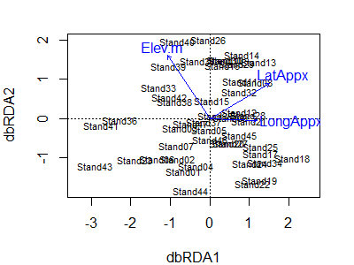
Notes:

• The first two axes are shown by default. If two or more axes are constrained, these are what will be shown.  If the dbRDA was based on a single explanatory variable with one df (i.e., only one constrained axis), the constrained axis and the first unconstrained axis will be shown.
• The vectors show the direction in which each explanatory variable is most strongly associated with the axes.
• The location of each sample unit is shown by its name.

Unconstrained Axes

The unconstrained axes are the result of a PCA on the residuals (i.e., variation that was not related to the set of explanatory variables).

The unconstrained axes are named differently to distinguish them from the constrained axes.  Furthermore, recall that a PCoA can produce negative eigenvalues if the underlying distance matrix does not satisfy the triangle inequality.  As a result, two types of unconstrained axes are reported:

• MDS1, MDS2, etc. – unconstrained axes associated with positive eigenvalues
• iMDS1, iMDS2, etc. – unconstrained axes associated with negative eigenvalues (the ‘i’ refers to ‘imaginary’)

The unconstrained axes are generally not the topic of interest in a dbRDA.  Do you see why?

Interpreting RDA and dbRDA

RDA uses Euclidean distances, so it is most appropriate when this distance measure is appropriate for the response matrix.  If no constraining variables are included, the result is a regular PCA.

Although RDA and dbRDA begin with a multivariate linear regression linear model, Borcard et al. (2018, ch. 6.3.2.10) note that it is possible to also test second-degree (i.e., quadratic) variables.  This can be useful if responses are unimodal, for example.

A major difficulty with all constrained ordinations is choosing which explanatory variables to constrain the ordination with.  Model-testing and model-building functions can be applied to identify the optimal set of explanatory variables to include.  See Borcard et al. (2018, ch. 6.3.2.6) for details.  As more constraining variables are included, the model ends up increasingly behaving like an unconstrained ordination because there is more flexibility within the constraints.

Finally, note that the set of explanatory variables is considered en masse; the loadings demonstrate how the score on each constrained axis is a linear combination of those explanatory variables.  These techniques are therefore not designed to evaluate which explanatory variables would be important if considered independently.

Conclusions

Several of these techniques are closely related.  For example, a RDA without constraining explanatory variables is a PCA, and a dbRDA without constraining explanatory variables is a PCoA.

RDA does not have CCA’s issues related to the use of the chi-square distance measure, though it does assume Euclidean distances and therefore is appropriate for variables where that distance measure is appropriate.  dbRDA can be applied to a distance matrix obtained using any distance measure.

References

Anderson, M.J., and T.J. Willis. 2003. Canonical analysis of principal coordinates: a useful method of constrained ordination for ecology. Ecology 84:511-525.

Borcard, D., F. Gillet, and P. Legendre. 2018. Numerical ecology with R. 2nd edition. Springer, New York, NY.

Legendre, P., and M.J. Anderson. 1999. Distance-based redundancy analysis: testing multispecies responses in multifactorial ecological experiments. Ecological Monographs 69:1-24.

Legendre, P., and L. Legendre. 2012. Numerical ecology. Third English edition. Elsevier, Amsterdam, The Netherlands.

Manly, B.F.J., and J.A. Navarro Alberto. 2017. Multivariate statistical methods: a primer. Fourth edition. CRC Press, Boca Raton, FL.

McArdle, B.H. and M.J. Anderson. 2001. Fitting multivariate models to community data: a comment on distance-based redundancy analysis. Ecology 82:290-297.