There is a growing concern in science about the extent to which it is reproducible.  In biomedical studies, for example, the strain of organism or conditions in the lab can have much larger effects than were previously appreciated (e.g., Lithgow et al. 2018).  In ecology, these concerns recently led to the formation of the Society for Open, Reliable, and Transparent Ecology and Evolutionary Biology (SORTEE).

A similar issue relates computationally.  An individual analysis requires hundreds of large and small decisions, and some of those decisions can dramatically affect the conclusions.  Computational reproducibility should be easier to demonstrate than reproducibility in lab environments.  Kitzes et al. (2018) state that “a research project is computationally reproducible if a second investigator (including you in the future) can recreate the final reported results of the project, including key quantitative findings, tables, and figures, given only a set of files and written instructions.”  Ideally, the script you produce for this course will fit this description!  Filazolla & Lortie (2022) provide recommendations for writing clean code.

The field of data science has much to teach us about computational reproducibility.  Options even exist to analyze R code directly (McGowan et al. 2020).

Analysis Organization

Projects

RStudio uses projects to help organize analyses.  Specifically, a project is self-contained and provides access to data, scripts, etc.  We will follow this approach.  For additional details, see Robinson (2016) and Bryan (2017).

The main directory for the project is the working directory.  This is where R will automatically look for files, and where files that are produced will automatically be saved. This also provides portability, as the project file will be useable by a collaborator even if their directory structure differs from yours.

When you open a R project, the working directory is automatically set as the folder in which the project file is stored.  You can confirm the working directory using the getwd() function:
getwd()

Note: one advantage of using a R project is that the working directory is automatically set.  If needed, however, you can use the setwd() function to change the working directory. You can specify a particular folder by typing out the address, or you can use the choose.dir() function to open a window through which you can navigate to the desired folder.
setwd("C://Users/jbakker/Desktop/SEFS 502/")
setwd(choose.dir())

Note that the slashes that map out the folder hierarchy are the opposite of what is conventionally used in Windows.

Create a folder in which you will store all files associated with SEFS 502 class notes and examples.  Once you’ve created this folder, save a R project within it.  Use this project to open R and work through class examples.

Sub-folders

A key advantage of setting a working directory is that it allows a project to have a stable starting point yet to remain organized by having items in the appropriate sub-folders.  Commonly used sub-folders include:

• data
• graphics
• images
• library
• notes
• output
• scripts (note: most data scientists now would recommend that you store your scripts on GitHub. See ‘Workflow design’ below for more details)

From the working directory, you can navigate using the relative path of a file rather than its absolute path. Sub-folders are referenced by simply including them in the name of the file you are accessing. For example, if the file ‘data.csv’ was stored in the data sub-folder, we could open it like this:
dataa <- read.csv("data/data.csv", header = TRUE, row.names = 1)

Using relative paths keeps your code portable among machines and operating systems (Cooper & Hsing 2017).  However, note that you do need to have the same sub-folders in your project folder.

In the folder that contains your SEFS 502 class project, create the following sub-folders:

• data
• scripts
• functions
• graphics

You can also create additional sub-folders, such as one for class notes, one for readings, etc. if desired.

Project Options

RStudio allows you to save your history (record of code that was run previously) and the objects that were created earlier.  However, I advise against this because these shortcuts increase the chance of errors creeping in.  For example, objects created during earlier sessions are still available for manipulation even if the current version of the script does not create them.

To turn these options off in RStudio, go to the ‘Tools’ menu and select ‘Project Options’.  Under the ‘General’ settings, set these options to ‘No’:

• Restore .RData into workspace at startup
• Save workspace to .RData on exit
• Always save history (even if not saving .RData)

Scripting

R Scripts

Scripting is one of the powerful aspects of R that distinguishes it from point-and-click statistical software.  When a script is clearly written, it is easy to re-run an analysis as desired – for example, after a data entry error is fixed or if you decide to focus on a particular subset of the data.  To capitalize on this ability, it is necessary to be able to manipulate your data in R.  New users often want to export their data to Excel, manipulate it there, and re-import it into R.  Resist this urge.  Working in R helps you avoid errors that can creep in in Excel – such as calculating an average over the wrong range of cells – and that are extremely difficult to detect (Broman & Woo 2018).

A script is simply a text file containing the code used (actions taken), along with comments clarifying why those actions were taken.  I save these files with a ‘.R’ suffix to distinguish them from other text files.  Scripts can be created within RStudio’s editor pane (my preference) but could also be created in R’s Editor or even in a simple text editor like WordPad.  Commands have to be copied and pasted into R for execution.

A script can include many different elements, including:

• Data import
• Define functions that will be used elsewhere (later) in the script
• Data adjustments
• Analysis
• Graphing

These elements can be organized in several ways.  In RStudio, for example, you can organize your code into sections.  Sections can be inserted via the ‘Code -> Insert Section’ command, or you adding a comment that includes at least four trailing dashes (—-), equal signs (====), or pound signs (####).

You can use the ‘Jump to’ menu at the bottom of the script editor to navigate between sections.

Individual sections can be ‘folded’ (minimized) to make the overall structure more apparent. The code within that section is replaced with an icon consisting of a blue box with a bidirectional arrow in it.  This is also helpful because you can select and run the entire folded section simply by highlighting the symbol that icon.

If your script includes multiple sections:

• Alt-O minimizes all sections
• Alt-Shift-O maximizes all sections

Interactive Notebooks (Jupyter, RMarkdown)

Interactive notebooks provide the capability to create a single document containing code, its output (statistical results, figures, tables, etc.), and narrative text.  They have been getting a lot of attention recently.  Key advantages are that the connections between data and output are explicit, and the output is automatically updated if the data change.

There are two broad types of interactive notebooks:

• Project Jupyter creates a file that contains the code, output, and narrative text.  This file is not of publication quality but is helpful for sharing an analysis with collaborators.  UW is testing opportunities to use JupyterHub for teaching; see the link in Canvas if you want to explore or use this.  Please note that this course’s JupyterHub workspace is only active for this quarter, so if you use it you will need to download any files that you wish to keep at the end of the quarter. 
• RMarkdown: A RMarkdown file consists of code and narrative text; Tierney (2020) provides a nice overview of RMarkdown and how to use it.  The code can include instructions to create figures or tables.  When this file is processed, the output specified by the code is produced and the resulting document is saved as a .pdf or .html file.  As such, this approach is closely aligned with publication – in fact, Borcard et al. (2018) state that their entire book was written using RMarkdown in RStudio!  (I considered creating these notes in RMarkdown but apparently it doesn’t integrate with the PressBooks publishing platform).

Workflow Design

Ecologists (myself included) are rarely trained as programmers, but knowing some of the ‘best practices’ that programmers use can improve the quality of our scripts.  Examples of these practices include:

• Modularizing code (i.e., writing custom functions) rather than copying and pasting it to apply it to different objects.  This prevents errors where you update the code in one location in your script but forget to update it elsewhere.  Modularizing code is also helpful for maintaining consistency.  For example, imagine that you want to create multiple figures with a consistent format.  If the script is written as a function, it can be called multiple times with different data.  Formatting details would remain the same from figure to figure.  And, if you decided to adjust the formatting you would only have to do so in one place!
• Verifying that code is working correctly via assertions and unit tests (automated testing of units of code)
• Version control to keep track of changes.  Many (most?) data scientists use Git for this purpose.  Closely associated with this is GitHub, which enables code sharing.  The data files for this book are available in the course’s GitHub repository (https://github.com/jon-bakker/appliedmultivariatestatistics).

Cooper & Hsing (2017) is an excellent resource in this regard.  There is also a growing body of open-source resources (free on-line lessons; in-person workshops at various locations) available through Software Carpentry.  And, the ‘Happy Git with R’ website appears to be quite readable and useful.

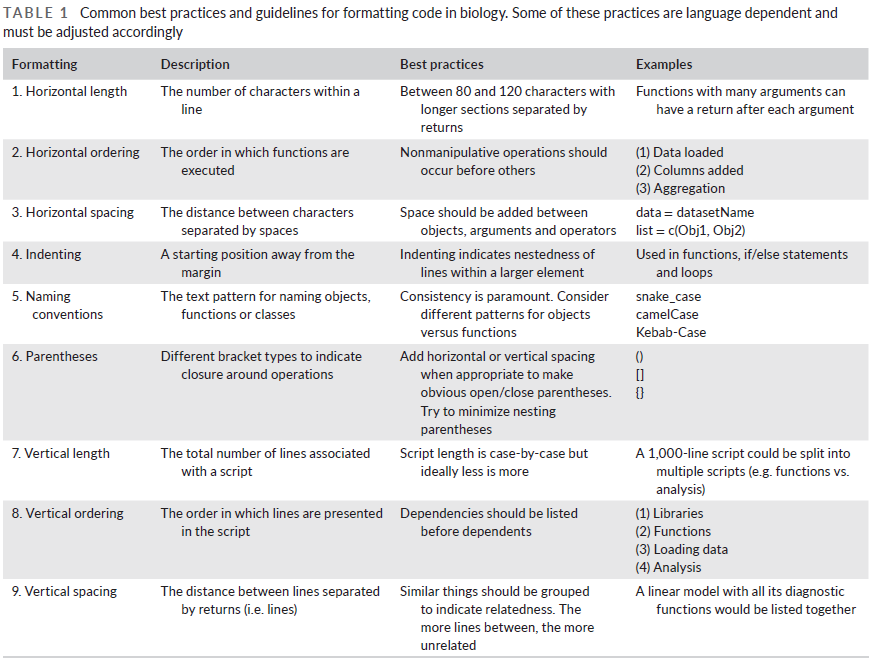
Some best practices and guidelines for formatting code are provided in Table 1 below.

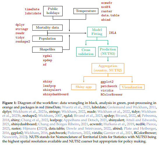
McCune & Grace (2002; ch. 8) provide a flowchart and tabular techniques that can assist in this process.  See this Appendix for a summary.  Workflows can be described verbally or graphically, as in this example:

Conclusions

The scientific process is built on the idea of reproducibility, both in the field and at the computer.  The ability to script an analysis is essential to ensuring that analyses can be shared and repeated.

References

Borcard, D., F. Gillet, and P. Legendre. 2018. Numerical ecology with R. 2nd edition. Springer, New York, NY.

Broman, K.W., and K.H. Woo. 2018. Data organization in spreadsheets. The American Statistician 72(1):2-10.

Bryan, J. 2017. Project-oriented workflow. https://www.tidyverse.org/blog/2017/12/workflow-vs-script/

Cooper, N., and P-Y. Hsing. 2017. A guide to reproducible code in ecology and evolution. British Ecological Society, London, UK. http://www.britishecologicalsociety.org/wp-content/uploads/2017/12/guide-to-reproducible-code.pdf

Filazzola, A., and C.J. Lortie. 2022. A call for clean code to effectively communicate science. Methods in Ecology and Evolution 13:2119-2128.

Kitzes, J., D. Turek, and F. Deniz (eds.). 2018. The practice of reproducible research: case studies and lessons from the data-intensive sciences. University of California, Oakland, CA. http://www.practicereproducibleresearch.org/

Konstantinoudis, G., V. Gómez-Rubio, M. Cameletti, M. Pirani, G. Baio, and M. Blangiardo. 2023. A workflow for estimating and visualising excess mortality during the COVID-19 pandemic. The R Journal 15(2):89-104.

Lithgow, G.J., M. Driscoll, and P. Phillips. 2018. A long journey to reproducible results. Nature 548:387-388.

McCune, B., and J.B. Grace. 2002. Analysis of ecological communities. MjM Software Design, Gleneden Beach, OR.

McGowan, L.D., S. Kross, and J. Leek. 2020. Tools for analyzing R code the tidy way. The R Journal 12:226-242.

Robinson, A. 2016. icebreakeR. https://cran.rstudio.com/doc/contrib/Robinson-icebreaker.pdf

Tierney, N. 2020. RMarkdown for scientists. https://rmd4sci.njtierney.com/