Introduction

After covering some foundational concepts, we covered topics that fall into three main categories:

• Testing for differences among a priori groups
• Identifying groups within your data (classification)
• Visualizing multivariate data

For example, you might use PERMANOVA to identify a difference in composition between levels of a factor, or you might use a hierarchical cluster analysis to identify groups of plots that are similar to one another in terms of their distances.  After applying either technique, you might then conduct an ordination to show the overall patterns across the set of response variables.

However, what else can you do to figure out what the multivariate patterns mean?

A Multivariate Test as an ‘Insurance Policy’

If you conduct enough statistical tests, you will find something statistically significant.  A multivariate test can serve as an insurance policy that reduces the chances of such spurious patterns.  Recall that we are testing the multivariate set of responses simultaneously.  If a multivariate test is not significant, there is no justification to test each univariate response.

A statistically significant multivariate test is an indication that there are patterns to be explored and understood.  However, multivariate tests don’t show you directly which response variable(s) are driving the patterns.  For example, patterns could be the net effect of small changes in many response variables, or could reflect large changes in a small number of response variables.  Furthermore, some response variables may be affected by one explanatory variable while others are affected by a different explanatory variable.

Decisions about how to analyze individual response variables should incorporate the characteristics of the data.  In this context, the key distinction is between non-compositional and compositional data.

Non-Compositional Data

Non-compositional data are generally continuously distributed and have few zeroes – each variable has a measured value in each sample unit.

If response variables are strongly correlated with one another, it is often helpful to capitalize on the fact that eigen-based techniques create new synthetic variables that are uncorrelated with each other.  For example, although every principal component (PC) is a linear combination of the original variables, by definition they are uncorrelated with the other PCs from that eigenanalysis.  This means that each PC can be interpreted separately and analyzed independently.

Continuously-distributed response variables that are not strongly correlated with one another are often analyzed using a separate linear model for each variable.  Furthermore, techniques like PERMANOVA and RRPP can be applied identically to both multivariate and univariate data, greatly simplifying follow-up analyses – the response changes but the structure of the model does not change.

Compositional Data

Compositional data (e.g., abundances of taxa within communities) are different from many other types of data.  In particular, the matrix is often sparse (i.e., contains many zeroes).  These absences are part of the patterns exhibited by individual taxa.  If we simply calculate an average abundance for each taxon in each group, we are potentially ignoring a lot of information about their distributions.

The chapters in this part survey several techniques to identify the species (response variables) associated with the observed patterns:

• Similarity percentage (SIMPER) – to identify the relative importance of each species in distinguishing between two levels of a categorical variable.
• Indicator Species Analysis (ISA) – to identify species that are strongly associated with (i.e., indicative of) one level or a set of levels of a categorical explanatory variable.
• Threshold Indicator Taxa ANalysis (TITAN) – to identify species that are strongly associated with low or high values of a continuous explanatory variable.

Other techniques are also possible – for example, Hu & Satten (2020) proposed a linear decomposition model that can both test for overall effects of a treatment and test whether individual taxa differ with respect to that treatment.  The software to do so is provided in their LDM package, and includes an alternate implementation of PERMANOVA.

Oak Example

We will use the oak plant community dataset to illustrate these follow-up tests.  Use the load.oak.data.R script to load and make initial adjustments to the oak plant community dataset.

source("scripts/load.oak.data.R")

The resulting object, Oak1, contains abundances of the 103 most abundant species, each relativized by its maxima.

Categorical Explanatory Variable (Grazing)

To illustrate the ideas below, we’ll use an explanatory variable that identifies the combined grazing status – past and current – of each stand.  There are three combinations of these grazing statuses.  We used these combinations in previous notes, but the levels had unhelpful names (e.g., ‘No_No’); let’s give them more intuitive names this time.

Oak_explan <- Oak_explan %>%
rownames_to_column(var = "Stand") %>%
rowid_to_column(var = "ID") %>%
mutate(GP_GC = paste(GrazPast, GrazCurr, sep = "_")) %>%
merge(y = data.frame(GP_GC = c("No_No", "Yes_No", "Yes_Yes"),
Grazing = c("Never", "Past", "Always"))) %>%
arrange(ID)

Note that we end this code by arranging the rows by ID to ensure that they remain in the same order as they are in our response matrix (Oak1).

summary(as.factor(Oak_explan$Grazing))

Always  Never   Past 
    17     24      6 

Does composition differ among grazing statuses?  We can test this via PERMANOVA:

set.seed(42)

adonis2(Oak1 ~ Grazing,
data = Oak_explan,
distance = "bray")

Permutation test for adonis under reduced model
Terms added sequentially (first to last)
Permutation: free
Number of permutations: 999

adonis2(formula = Oak1 ~ Grazing, data = Oak_explan, distance = "bray")
         Df SumOfSqs      R2      F Pr(>F)   
Grazing   2   0.9095 0.07844 1.8725  0.006 **
Residual 44  10.6854 0.92156                 
Total    46  11.5949 1.00000                 
---
Signif. codes:  0 ‘***’ 0.001 ‘**’ 0.01 ‘*’ 0.05 ‘.’ 0.1 ‘ ’ 1

Grazing treatments do differ in composition.

Let’s also visualize composition patterns and grazing treatments.  We’ll use NMDS here so that we see the grazing treatments in the context of all of the compositional variation expressed in these dimensions:

source("functions/quick.metaMDS.R")

set.seed(42)

Oak.nmds <- quick.metaMDS(Oak1, 3)

library(ggvegan)

Oak.nmds.gg <- fortify(Oak.nmds) %>%
filter(score == "sites")

Oak_explan <- Oak_explan %>%
merge(y = Oak.nmds.gg, by.x = "Stand", by.y = "label")

theme.custom <- theme_bw() +
theme(axis.line = element_line(),
axis.ticks = element_blank(),
axis.text = element_blank(),
axis.title = element_blank())

ggplot(data = Oak_explan, aes(x = NMDS1, y = NMDS2)) +
geom_point(aes(colour = Grazing, shape = Grazing)) +
theme.custom

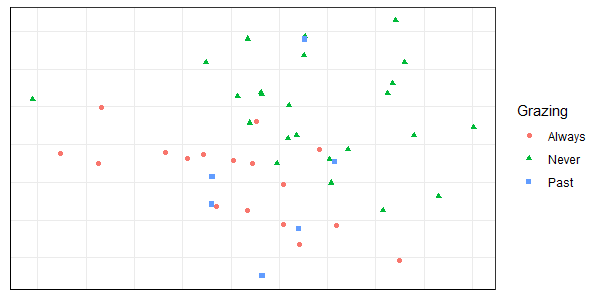
We’ll use SIMPER and ISA to explore which species are associated with these groups.

Continuously-Distributed Explanatory Variable (PDIR)

How does composition vary with light availability (PDIR)?  We can also analyze this with PERMANOVA:

set.seed(42)

adonis2(Oak1 ~ PDIR,
data = Oak_explan,
distance = "bray")

Permutation test for adonis under reduced model
Terms added sequentially (first to last)
Permutation: free
Number of permutations: 999

adonis2(formula = Oak1 ~ PDIR, data = Oak_explan, distance = "bray")
         Df SumOfSqs      R2      F Pr(>F)   
PDIR      1   0.8068 0.06958 3.3655  0.002 **
Residual 45  10.7881 0.93042                 
Total    46  11.5949 1.00000                 
---
Signif. codes:  0 ‘***’ 0.001 ‘**’ 0.01 ‘*’ 0.05 ‘.’ 0.1 ‘ ’ 1

Composition varies as a function of the light environment.

Now, let’s visualize how composition relates to light environment:

library(ggordiplots)

gg_ordisurf(ord = Oak.nmds, env.var = Oak_explan$PDIR)

(note that we can’t customize a gg_ordisurf() object the same way we can with regular ggplot2 objects)

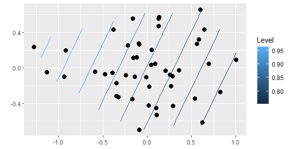
Sample units on one end of the ordination space tend to have higher light availability than those on the other end of the ordination space.  We’ll use TITAN to explore the species associated with these differences.

Conclusions

This is a brief introduction to a large topic.  How these techniques are used will have to reflect the details of your study.

References

Hu, Y-J., and G.A. Satten. 2020. Testing hypotheses about the microbiome using the linear decomposition model (LDM). Bioinformatics 36:4106-4115.