
Ordinations (Data Reduction and Visualization)
38 NMDS
Learning Objectives
To demonstrate how the NMDS algorithm works.
To consider when NMDS is an appropriate ordination technique.
To demonstrate how the fit of a NMDS ordination can be assessed.
To continue creating graphical images of ordinations.
Reading (Recommended)
Clarke (1993, p. 117-126)
Key Packages
require(vegan, tidyverse)
Introduction
Non-metric MultiDimensional Scaling (NMDS) is a distance-based ordination technique. Because it focuses on the distance matrix, it is very flexible – any distance measure can be used. As usual, the data matrix (n sample units × p species) is converted into an n x n distance matrix (or, more generally, a dissimilarity matrix).
Note: you will likely encounter a variety of abbreviations for Non-metric MultiDimensional Scaling (NMDS). People variously refer to it as non-metric MDS or NMS or MDS. I do not recommend this last abbreviation for NMDS, as it is also used to for metric MultiDimensional Scaling (aka PCoA), which we consider separately.
Characteristics of NMDS
NMDS was first popularized in the psychological literature (Shepard 1962a,b; Kruskal 1964a,b). It can be used to obtain an ordination from any distance measure. As we’ve discussed numerous times, the distance matrix summarizes the differences among each pair of sample units in terms of any number of response variables.
NMDS generally does a good job at representing complex multi-dimensional data in a small number of dimensions (usually 2 or 3). As a result, it is often used for data reduction and visualization.
NMDS is sometimes used simply for data reduction. For example, Haugo et al. (2011) examined vegetation dynamics within mountain meadows from 1983 to 2009. They conducted a NMDS ordination of the meadow communities in 1983, and determined that the coordinates in this ordination space related to landscape context (landform, hydrology, and elevational zone). They therefore used these coordinates as explanatory variables in a subsequent analysis of how the vegetation changed between 1983 and 2009.
More commonly, NMDS is used for data visualization (which often requires data reduction). Most papers that use NMDS will show one or more ordinations produced by this technique.
Techniques such as PCA can sometimes be used in other ways, such as to rotate a data cloud so that axes are ordered in declining order of importance. I cannot think of any situation where we would be interested in using NMDS for this type of application.
NMDS differs in several important ways from other ordination techniques:
- As noted above, NMDS is a distance-based technique.
- NMDS does not plot the distances per se among sample units. Instead, it attempts to plot sample units in such a way that the distances among sample units in the ordination space are in the same rank order as the distances among sample units as measured by the original distance matrix. In other words, it attempts to choose coordinates so that sample units that are similar in ‘real life’ are close together in the ordination space and sample units that are dissimilar in ‘real life’ are far away from one another in the ordination space.
- It can proceed even if some distances are missing from the dissimilarity matrix.
- It does not seek to maximize the variability associated with individual axes of the ordination. As a result, the axes of an NMDS ordination are entirely arbitrary, and plots may be freely rotated, centered, or inverted to increase interpretability.
- It is iterative – the positions of the sample units in ordination space are adjusted through a series of steps.
- Due to its iterative nature, it is computationally intensive to run with very large samples.
- The user must specify how many dimensions are desired for the solution. Solutions can differ depending on the number of dimensions selected: a 2-D solution may not be the same as the first two dimensions of the 3-D solution.
- There is no single solution.
NMDS In Action
It’s more difficult to discuss the theory behind NMDS than to see it in action. Let’s explore the process of doing a NMDS as illustrated in this video. Here’s a screenshot from the start of the video:
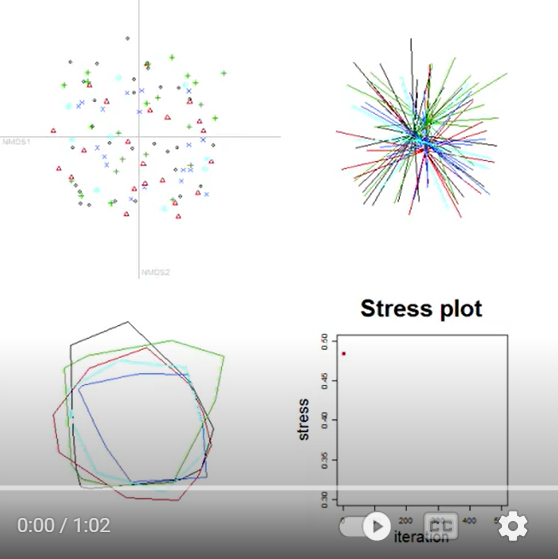
This image contains four graphics:
- Top left – the ordination space, with each sample unit shown as a point. Symbol shape and color distinguish the groups for illustration purposes.
- Top right – the ordination space, with each sample unit connected to the centroid of the group to which it belongs. This type of image is called a ‘spider’.
- Bottom left – the ordination space, with a perimeter (hull) encompassing all of the sample units from each group.
- Bottom right – a ‘stress plot’ showing how model fit, as measured by stress (see below), changes iteratively.
It is important to note that group identity is shown for illustration purposes. The NMDS algorithm proceeds on the basis of the distance matrix, and is not influenced by group identity.
Initially, the sample units are positioned at random starting coordinates in the 2-D ordination space. As a result, the points are interspersed and the spiders and hulls of the different groups are indistinguishable.
The NMDS algorithm involves calculating the distances between sample units in the ordination space, comparing these distances to the distances based on the actual responses, and iteratively adjusting the coordinates of the sample units in the ordination space to increase the agreement between these two sets of distances (i.e., to lower the stress).
Here is a screenshot from the end of this process – in this case, after 500 iterations:
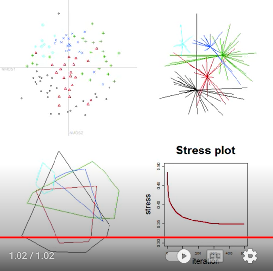
Observe how sample units from different groups tend to occur in different locations within the two-dimensional ordination space. This separation was based on the values in the distance matrix, not on the group identities. Group identity was used to distinguish observations within this example, but is not ‘known’ to the NMDS algorithm.
NMDS in R (vegan::metaMDS())
NMDS can be conducted using several functions in R. We will use the functions available in the vegan package; others include MASS::sammon(), ecodist::nmds(), and smacof::mds(). Functions often differ in argument names and may differ in other aspects (e.g., choice of initial coordinates), so be sure to check the appropriate help files if using other functions.
The vegan package uses monoMDS() as its ‘workhorse’ NMDS function. The arguments of this function allow us to control the details of the NMDS ordination. Additional functions process the data file before it can be used by monoMDS() and process the results afterwards. These individual functions can also be called directly if you want to retain maximal control of all aspects of the NMDS process. However, it is more common to use a ‘wrapper’ function, metaMDS(), which has the advantage of also calling these other functions before and after monoMDS(). This function is structured to follow the recommendations of Minchin (1987). For example, metaMDS():
- Allows a data matrix to be specified (in comparison,
monoMDS()requires a distance matrix) - Can automatically decide whether/how to transform the data
- Can automatically decide which type of distance measure to use
When calling other functions (e.g., vegdist() to convert a data matrix to a distance matrix); the defaults of those functions apply unless overwritten using arguments within metaMDS().
The help file for metaMDS() shows the many arguments that are part of its usage. Here, I have organized the key arguments within the steps of a NMDS ordination, including the wrap-around functions. If arguments have defaults, they are identified here as well. I have highlighted key settings in bold.
Pre-NMDS (Initial) Steps
Begin with comm, a community data matrix (n sample units × p species) or a n × n distance matrix. If a distance matrix is specified, the rest of the pre-NMDS steps are skipped.
Transform data matrix if autotransform = TRUE. The sqrt() transformation is applied if the maximum value in comm is ≤ 50 and wisconsin() standardization is applied if the maximum value in comm is > 9. However, as noted in the help file, these criteria are arbitrary. To ensure clarity and control of the analysis procedure, I recommend doing desired transformations and/or standardizations before using metaMDS(). I therefore recommend setting autotransform = FALSE.
Convert the data matrix to a distance matrix, using an appropriate distance measure. This calls vegdist() and uses its default of the Bray-Curtis distance (distance = "bray"), but any distance measure available in that function can be called here. If you want to use a distance measure that is not available within vedist(), calculate the distance matrix using another function and specify it as comm.
Choose which engine (function) to conduct the NMDS with. The default, engine = "monoMDS", is assumed in these notes. The alternative, engine = "isoMDS", is included here for backward compatibility with early versions of vegan that did not contain monoMDS().
Choose how to deal with long environmental gradients. Recall that the Bray-Curtis distance measure (and related measures) have an upper bound of 1 if two sample units do not share species. If the compositional data span a long environmental gradient such that many sample units do not share species, it can be difficult to identify patterns as some sample units are completely different from many other sample units. There are two ways to deal with this, depending on the engine used:
- If the default engine is being used (
engine = "monoMDS"), theweaktiesargument allows observations with identical dissimilarities to have different fitted distances (weakties = TRUE). In other words, settingweakties = TRUEallows observations to be positioned at different coordinates within the ordination space even though they are the same distance apart in the distance matrix. Settingweakties = FALSEforces observations that are the same distance apart in the distance matrix to also be the same distance apart in ordination space. - If the alternative engine is being used (
engine = "isoMDS"), extended dissimilarities can be calculated using thenoshareargument, which calls thestepacross()function. Extended dissimilarities incorporate paths that include ‘intermediate’ sample units – those that share some species with two sample units that do not share species directly (De’ath 1999). Using extended dissimilarities has implications that have not been fully explored, including the fact that the distance measure no longer has a constant upper bound. The argument default isnoshare = (engine == "isoMDS")– this looks confusing but is simplyTRUEif isoMDS has been specified andFALSEotherwise.
NMDS Steps
1. Specify how many dimensions (k) you want the solution to contain. Note that you will get a different result if you use different values of k! In the help files, it is recommended that you have at least twice as many sample units as dimensions (though this recommendation is trivial in most situations).
2. Assign a starting configuration (y) to sample units. This can be done many ways:
- Randomly assign starting coordinates to sample units. This is the default in
monoMDS(). - Use results of another ordination (e.g., PCA, PCoA) as starting coordinates. For example, set
y = cmdscale(d, k)to do a PCoA ordination ofdinkdimensions. This is the default inmetaMDS(). - Use the
previous.bestargument to begin with the best solution from a previous run ofmetaMDS(). - If data are spatially structured, use the geographic position of each sample unit as its starting coordinates.
- Compute NMDS using (
k+ 1) dimensions. Use final coordinates from this ordination as the starting coordinates in a run usingkdimensions.
3. Calculate Euclidean distances among sample units in the ordination space.
4. Compare the fitted distances from the ordination space with the distances in the original dissimilarity matrix (see ‘Evaluating Fit’ section below). The calculated goodness-of-fit of a regression between these distances is called the stress. Stress is usually calculated using monotone regression (i.e., based on the ranks of the data); this is done by setting model = "global". The other options ("local", "linear", "hybrid") allow you to use this function to conduct other types of NMDS. Stress is described in the ‘Stress’ section below. monoMDS() reports stress as a proportion (i.e., bounded between 0 and 1) and provides two ways to calculate it (1 or 2); stress = 1 is the standard option and the default.
5. Determine whether the fit is ‘good enough’. monoMDS() uses three different stopping criteria to determine whether changes in configuration are improving fit. In my experience, these stopping criteria generally do not require adjustment. They are:
smin = 1e-4: stop when stress drops below this valuesfgrmin = 1e-7: stop when ‘minimum scale factor’ (I’m not sure how this is calculated) is below this valuesratmax = 0.999999: stop when stress ratio exceeds this value
6. If none of the stopping criteria have been met, improve the configuration by moving sample units in a direction that will reduce the stress. This is done using a method called ‘method of steepest descent’. Basically, the idea is to shift coordinates in the manner that will cause the greatest reduction in the stress. The amount to move the configuration is determined by the step length; this value is recalculated after each iteration and gets smaller as the stress declines. McCune & Grace (2002, p. 128) describe a landscape analogy for NMDS that may be helpful for understanding this.
7. Repeat from step 3 until either:
- Convergence has been achieved.
- The maximum number of permitted iterations (
maxit = 200) have been performed. McCune & Grace (2002, Table 16.3) recommend a maximum of 400 iterations for configuration adjustments.
8. A single NMDS run identifies a local minimum, but this is not necessarily the global minimum. New runs help assess this. Each new run involves creating new random initial coordinates (step 2) and rerunning steps 3-7. The stress associated with the final configuration of the new run is compared to that from the initial run. If the new run resulted in a smaller stress, its configuration is saved as the new final configuration. This is repeated at least try = 20 times, and up to trymax = 20 times, or until the convergence criteria are met. McCune & Grace (2002, Table 16.3) recommend repeating this 40 times, though we can of course do more.
The trace = 1 argument causes the final stress value obtained from each run to be reported. Note that this can also be specified as trace = TRUE.
The default is to not display the results graphically (plot = FALSE). Changing this to plot = TRUE produces Procrustes overlay plots comparing each new solution with the previous best solution. We’ll discuss Procrustes analysis later.
9. Adjust final configuration:
- Center solution so that the centroid is at the origin.
- Rotate axes using PCA (
pc = TRUE). Allkaxes are kept, so this process rotates the data but does not alter its dimensionality. By definition, the resulting data cloud is oriented so that the first dimension expresses as much variation as possible, the second as much of the remaining variation as possible, etc. Alternatively, the final configuration can be rotated to align with an environmental variable usingMDSrotate()– we’ll illustrate this later. - Re-scale ordination axes to ‘unit root mean squares’ (
scaling = TRUE). Note that we generally do not pay much attention to the scales of the axes, however.
Adopt the coordinates of each sample unit from the final configuration as its coordinates in the k-dimensional ordination space.
Post-NMDS Steps
Calculate species scores as the weighted average of the coordinates of the plots on which those species occurred. This argument (wascores = TRUE) simply calls wascores(). See the ‘Species Scores’ section below for details.
Oak Example
Let’s conduct a NMDS on the oak plant community dataset.
Use the load.oak.data.R script to load and make initial adjustments to the oak plant community dataset. Although this script calculates a distance matrix, we will work with the intermediate object Oak1, which contains abundances of the 103 most abundant species, each relativized by its maxima. Using this data matrix allows us to see how to control the initial (pre-NMDS) options within metaMDS().
source("scripts/load.oak.data.R")
Conduct a NMDS. For completeness, I will specify they key arguments here even though I want to use their default settings. Doing so avoids potential issues if the default would change, for example.
To ensure results are repeatable, we’ll set the random number generator immediately before doing so. You’re welcome to explore the extent to which altering the random number generator changes the results.
set.seed(42)
z <- metaMDS(comm = Oak1,
autotransform = FALSE,
distance = "bray",
engine = "monoMDS",
k = 3,
weakties = TRUE,
model = "global",
maxit = 300,
try = 40,
trymax = 100)
The resulting object is of class ‘metaMDS’. The summary() for an object of this class is not that informative, but we can use print() to see a summary of what was done:
print(z)
Call:
metaMDS(comm = Oak1, distance = "bray", k = 3, try = 40, trymax = 100,      engine = "monoMDS", autotransform = FALSE, weakties = TRUE,      model = "global", maxit = 300)

global Multidimensional Scaling using monoMDS

Data:     Oak1
Distance: bray

Dimensions: 3
Stress:     0.1641748
Stress type 1, weak ties
Best solution was repeated 7 times in 40 tries
The best solution was from try 0 (metric scaling or null solution)
Scaling: centring, PC rotation, halfchange scaling
Species: expanded scores based on ‘Oak1’
We can also use str() to explore the object and identify particular items of interest. Those items include:
- Stress value of solution –
z$stress - Coordinates of each sample unit in the k-dimensional ordination space –
z$points. These coordinates can also be extracted usingscores(z). - Coordinates of each species in the k-dimensional ordination space –
z$species. Only available ifwascores = TRUEduring analysis. - The distances between sample units in the original distance matrix –
z$diss. - The distances between sample units in the ordination space –
z$dist.
Stress
Stress can be calculated using several formulae (McCune & Grace 2002, p. 126-127). However, stress formulas generally yield similar configurations. In R, stress is reported as a proportion (0-1) or a percent (0-100). The default formula in monoMDS() is:
[latex]S = \sqrt{\frac{\sum_{i=1}^{n-1} \sum_{j=i+1}^n (d_{ij} - \tilde d_{ij})^2} {\sum_{i=1}^{n-1} \sum_{j=i+1}^n d_{ij}^2}}[/latex]
where [latex]d_{ij}[/latex] is the distance in the original dissimilarity matrix and [latex]\tilde d_{ij}[/latex] is the fitted distance in ordination space. This formula is what is used when stress = 1; when stress is calculated using the alternative formulation (stress = 2), the denominator is adjusted; see ?monoMDS for details.
As noted in the last section, the stress achieved by the final solution of a NMDS is part of the resulting object:
z$stress
0.1641748
Is this good? Clarke (1993, p. 126) suggests the following rules of thumb for stress values:
| Stress (0-1 scale) | Interpretation |
| < 0.05 | Excellent representation with no prospect of misinterpretation |
| < 0.10 | Good ordination with no real disk of drawing false inferences |
| < 0.20 | Can be useful but has potential to mislead. In particular, shouldn’t place too much reliance on the details |
| > 0.20 | Could be dangerous to interpret |
| > 0.35 | Samples placed essentially at random; little relation to original ranked distances |
While these rules of thumb are useful, they’re guidelines rather than absolutes. In particular, the stress of a given solution is a function of:
- Sample size – “the greater the number of samples, the harder it will be to reflect the complexity of their inter-relationship in a two-dimensional plot” (Clarke 1993, p. 125).
- Nature of data – is stress attributable to all points or to a single one that isn’t easily placed?
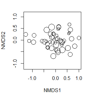
One way to explore the effect of individual points is with the goodness() function:
gof <- goodness(object = z)
The resulting vector summarizes the proportion of the overall variance that is explained by each sample unit. An extremely large value would be an indication that a sample unit is causing a poor fit in the ordination – perhaps there is something unique about it? I’ve also had times when a data entry error caused one sample unit to appear hugely different from all of the others. We can visualize these statistics:
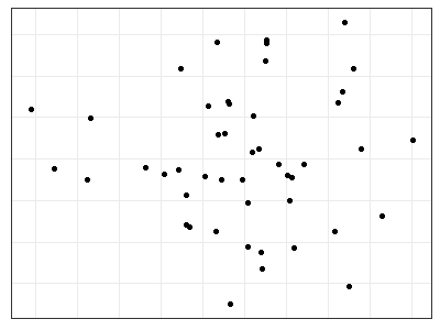
plot(z, display = "sites", type = "none")
points(z, display = "sites", cex = 2*gof/mean(gof))
Note that the cex (character expansion) argument looks complicated but is just sizing each symbol to be proportional to its value relative to the mean of them all. Sample units shown with larger circles account for more of the variation in the overall fit of these data.
Evaluating Fit
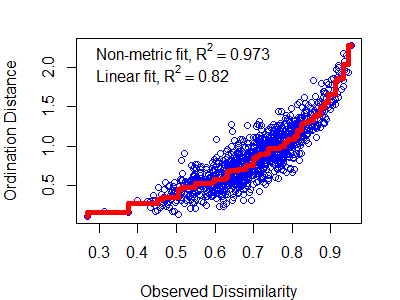
The fit of a NMDS ordination can be assessed by plotting the original dissimilarities (z$diss) against the (Euclidean) ordination distances (z$dist). The number of distances and dissimilarities increases rapidly with the number of sample units (N): recall that each matrix contains N(N – 1)/2 pairwise elements. Also, the process of comparing two distance matrices should remind you of a Mantel test.
A plot of dissimilarities vs. ordination distances is known as a Shepard plot (see Fig. 2 in Clarke 1993). It can be created manually:
plot(z$diss, z$dist)

You can calculate the distances directly from the data to verify that the mapped values in the Shepard plot are from the original data and the coordinates in the ordination space:
#plot(vegdist(Oak1), dist(scores(z, "sites"))) #compare to above
Shepard plots can also be created using the stressplot() function in vegan. One advantage of this over the manual approach is that it also adds a fit line (a non-linear step function) and two ‘correlation-like’ statistics:
- Non-metric or monotonic fit – calculated as 1 –
z$stress^2. - Linear fit – squared correlation between fitted values and ordination distances.
The usage of stressplot() is:
stressplot(object,
dis,
pch,
p.col = "blue",
l.col = "red",
lwd = 2,
...
)
The arguments are:
object– the output of ametaMDS(),monoMDS(), orisoMDS()function.dis– dissimilarities. Only required if object is fromisoMDS().pch– plotting character for points. Default is dependent on the number of points.p.col– point color. Default is blue.l.col– line color. Default is red.lwd– line width.
stressplot(object = z, lwd = 5) # Thicker line
Graphing the Final Configuration
A unique element of graphing a NMDS ordination is that the axes cannot be interpreted like those in a PCA – instead, the focus is on the data points themselves, and particularly on their orderings relative to one another. Therefore, NMDS ordinations are often plotted without units or labels on the axes so that people do not try to interpret them.
Obtaining the Ordination Coordinates
To graph a NMDS ordination (or any other object!), we need to know where the coordinates are stored. As noted above, the str() function is a good starting point. In this case, the coordinates are saved as points in the object.
z$points %>% head()
               MDS1        MDS2       MDS3
Stand01 -0.39411569 -0.05254510  0.3604700
Stand02 -0.34549234 -0.17365891  0.2593316
Stand03 -0.23802128 -0.08292349  0.1002232
Stand04 -0.09426964  0.27745268  0.1299250
Stand05  0.82431684 -0.27299339 -0.4049859
Stand06 -0.47766863 -0.07318759 -0.2589466
These coordinates are the positions of each sample unit in the ordination space. Points near one another are similar in their multivariate response, while points far from one another are different in their multivariate response.
We can either call the coordinates directly, save them to a new object, or combine them with the raw data or the other explanatory variables. Here, I’ll save them to their own object:
z.points <- data.frame(z$points)
Using ggplot2
Once we have the coordinates of the points, we can graph the ordination using ggplot2. In this case, I’m going to save the formatting aspects of this code as its own object so that I can easily re-use it below.
p <- ggplot(data = z.points, aes(x = MDS1, y = MDS2)) +
theme_bw() +
theme(axis.title = element_blank(),
axis.ticks = element_blank(),
axis.text = element_blank())
p + geom_point()
General Notes about Visualizations
Recall that axes were rotated via PCA as the last step in the NMDS algorithm in metaMDS(). As a result, the axes are arranged so that they explain declining amounts of variation. We graphed the first two axes above, but it is important to remember that the axes in a NMDS do not have an inherent meaning like they do in PCA. It therefore is perfectly acceptable to look at the NMDS data cloud from other perspectives. This can take several forms:
- Viewing other combinations of axes. Obviously, this is only possible if you have specified a solution with more than two axes! In
ggplot2, this is specified by changingxandy. - When comparing an ordination to an explanatory variable: rotate an ordination so that the first axis is parallel to the explanatory variable. This can be done using the
MDSrotate()function, which we’ll discuss later. - When comparing two ordinations based on data from the same sample units: orient them so that sample units from the same group are in the same relative location. Procrustes analysis is one method to do so.
Graphing with Base R Capabilities
We can use the plot() function to see a graph of the final configuration of the metaMDS results. By default, this function displays both sites and species. We can use the display argument to specify which of these we want. To display only sites:
plot(z, display = "sites")

An alternative is to specify, while plotting, whether to plot points (type = "p"; the default) or text (type = "t") or neither (type = "n"; a blank graph).
Creating a blank graph is helpful if we want to customize it. We begin by creating a plot of z but not displaying any points and hiding the axis labels and units. The net result is that the axes are scaled to fit the data even though they aren’t shown. Then, we add the desired data as points(), text(), etc.
plot(z, display = "sites", type = "n",

xaxt = "n", xlab = "", yaxt = "n", ylab = "")
points(z, col = "red")

Species Scores
Calculations
NMDS coordinates show the locations of the sample units relative to one another, but what about the species?
One reason some people like ordination approaches such as correspondence analysis (CA) is that the mathematics result in coordinates for both the sample units and the species in the same ordination space. In CA, each species is plotted at the peak of its assumed unimodal response curve.
While we cannot do the same in NMDS, we can approximate the location at which each species is most abundant. To do so for a given species, we weight the coordinates of all plots by the abundance of that species in the plots. We can do so with the wascores() function:
sp <- wascores(x = z$points, w = Oak1, expand = TRUE)
The expand argument scales the species scores so that they have the same weighted variance as the scores of the sample units. This function could also have been called using the wascores argument in the post-NMDS step of metaMDS().
Personally, I have not found these species scores to be very useful. Knowing the weighted average score of each species doesn’t tell us, for example, whether a species is widespread or narrowly distributed. In my opinion, there are better ways to explore species. I illustrate some graphical techniques here, and also refer you to techniques such as Indicator Species Analysis and TITAN.
Graphing via ggplot2
Viewing all species at once is too busy to be interpretable (you’re welcome to try it out!). Let’s focus on two taxa, the shrubby and tree forms of Garry oak (Quga.s and Quga.t, respectively).
Quga <- data.frame(sp[c("Quga.s", "Quga.t"), ])
p +

geom_point() +

geom_text(data = Quga, label = rownames(Quga))

Note that we have added these to the graphic p that we created earlier. Do you agree that these two centroids aren’t too informative by themselves?
Let’s incorporate the actual data. We’ll make point sizes proportional to the abundance of Quga.s and Quga.t.
We begin by combining the NMDS coordinates with the abundance data for these species:
z.points <- data.frame(z.points,
Quga.s = Oak1$Quga.s,
Quga.t = Oak1$Quga.t)
Now we can use these abundance values in our graphing.
p +
geom_text(data = Quga, label = rownames(Quga),
colour = c("red", "blue")) +
geom_point(data = z.points[z.points$Quga.s > 0,],
aes(size = Quga.s), shape = 21, colour = "red") +
geom_point(data = z.points[z.points$Quga.t > 0,],
aes(size = Quga.t), shape = 21, colour = "blue") +
labs(size = "Abundance")
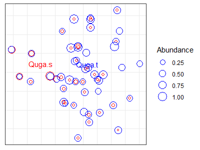
While creating this graph, I added the species scores (i.e., centroids) as text. I then plotted two sets of points, one for each species. For each set of points, I:
- restrict the data to non-zero values for that species
- made symbol size proportional to the relative abundance of the species
- used a different color
Issues in NMDS
How Many Dimensions to Use?
One of the key differences between NMDS and the other ordination techniques we’ve covered is that NMDS solutions are dependent on the number of dimensions selected. A 2-D solution differs from the first two dimensions of a 3-D solution. The number of dimensions is often selected by conducting NMDS ordinations with different numbers of dimensions (e.g., k = 1 to 5) and then plotting stress as a function of k. The intent here is to identify the point where adding the complexity of an additional dimension contributes relatively little to the reduction in stress.
How many dimensions are appropriate? The ‘correct’ answer is a balance between interpretive issues (interpretability of axes, ease of use, stability of solution) and statistical issues (stress):
- Too many axes defeats the purpose of visualizing and interpreting the dataset
- Too few axes can result in unacceptably large stress values
This subjectivity in terms of the number of dimensions is important to keep in mind because, as noted above, the axes of a NMDS ordination do not have the same interpretation as those in a PCA or CCA. Instead, the focus of NMDS is on the data points themselves, and particularly on their orderings relative to one another. As Clarke (1993) described it: “sample A is more similar to sample B than it is to sample C” (p. 117). For this reason, and as stated earlier, NMDS ordinations are often plotted without units or labels on the axes so that people do not try to interpret them.
The stress of a solution always decreases as the number of dimensions increases – adding another dimension means that there is more ‘room’ for adjustments in the coordinate space to increase the alignment between those distances and the original distance matrix.
Specifying more dimensions in a solution does not mean that you have to show them all graphically. For example, above we did a 3-dimensional NMDS but only displayed the first two dimensions. Since the coordinates were rotated via PCA, these dimensions show as much of the variation in the coordinates as possible in two dimensions. However, note again that the first two dimensions of a 3-dimensional solution are not the same as a 2-dimensional solution.
The significance of a solution can be assessed using Monte Carlo techniques to determine the likelihood of the observed stress values. To my knowledge, these techniques are not currently available in R (though it would be relatively easy to write a function that would perform these steps). The computational limitations of this technique have diminished greatly since McCune & Grace (2002) was published. Therefore, it is feasible to conduct more Monte Carlo tests than they recommend.
Unstable Solutions
Stress can be graphed as a function of the iteration number to assess fluctuations, stability, etc. This was shown in the YouTube video referenced earlier (see ‘NMDS in Action‘ section), but this type of graph is not available in the current NMDS functions in R. I have not yet found a way to track how stress changes with iteration number. The closest I am aware of is that the stress of the solution based on each random start is displayed on the screen (the trace = 1 argument in metaMDS()) but is not saved. The metaMDS() function could be altered to save this information…
Relation to Explanatory Variables
NMDS ordinations are based solely on a response matrix. We are often naturally very interested in comparing the resulting patterns to explanatory variables, both categorical (e.g., burned or not) and continuous (e.g., elevation). We can explore these relationships qualitatively by overlaying them onto the ordination – and will do so later. However, it is important to keep in mind when doing so that these patterns may be affected by how well the ordination fits the distance matrix. When overlaying explanatory variables onto an NMDS ordination, we are visualizing their relationship with the reduced dimensionality of the ordination space, not with the original distance matrix. In contrast, analytical techniques such as PERMANOVA quantify the relationship between explanatory variables and the distance matrix derived directly from the data.
Strengths and Interpretive Difficulties with NMDS
Strengths of NMDS:
- Avoids assumptions about form of relationships among variables
- Uses ranked distances to linearize relationships
- Allows use of any transformation, standardization, and distance measure. This allows the analytical methods to be determined by the ecology of the dataset. It also means that the ordination, formal tests of statistical significance (e.g., PERMANOVA, ANOSIM), and/or classification techniques (e.g., cluster analysis) can all use data that has received the same adjustments and thus are directly comparable with one another.
Interpretive Difficulties of NMDS:
- May fail to find the global solution (minimum stress)
- Slow computation with large datasets
- Interpretation is dependent on dimensionality of the ordination – which has to be specified by the user
- Based on the rank order of the distances, not on the distances themselves
Conclusions
Minchin (1987) compared PCA, PCoA, DCA, and NMDS, and concluded that NMDS is “a robust technique for indirect gradient analysis, which deserves more widespread use by community ecologists” (p. 89). McCune & Grace (2002) felt that NMDS and related techniques are the way ordination will be increasingly conducted in ecology. They noted that NMDS “is currently one of the most defensible techniques during peer review” (p. 125). von Wehrden et al. (2009) found that its usage increased between 1990 and 2007.
The relative differences among some of these models are unclear; Anderson (2015) notes that techniques like NMDS and PCoA will tend to give similar results, and that far more important differences arise from decisions about data adjustments (transformations, standardizations) and which distance measure to use.
References
Anderson, M.J., R.N. Gorley, and K.R. Clarke. 2008. PERMANOVA+ for PRIMER: guide to software and statistical methods. PRIMER-E Ltd, Plymouth, UK.
Anderson, M.J. 2015. Workshop on multivariate analysis of complex experimental designs using the PERMANOVA+ add-on to PRIMER v7. PRIMER-E Ltd, Plymouth Marine Laboratory, Plymouth, UK.
Anderson, M.J., and T.J. Willis. 2003. Canonical analysis of principal coordinates: a useful method of constrained ordination for ecology. Ecology 84:511-525.
Borcard, D., F. Gillet, and P. Legendre. 2011. Numerical ecology with R. Springer, New York, NY.
Clarke, K.R. 1993. Non-parametric multivariate analyses of changes in community structure. Australian Journal of Ecology 18:117-143.
De’ath, G. 1999. Extended dissimilarity: a method of robust estimation of ecological distances from high beta diversity data. Plant Ecology 144:191-199.
Gotelli, N.J., and A.M. Ellison. 2004. A primer of ecological statistics. Sinauer, Sunderland, MA.
Gower, J.C. 1966. Some distance properties of latent root and vector methods used in multivariate analysis. Biometrika 53:325-338.
Haugo, R.D., C.B. Halpern, and J.D. Bakker. 2011. Landscape context and tree influences shape the long-term dynamics of forest-meadow ecotones in the central Cascade Range, Oregon. Ecosphere 2:art91.
Kruskal, J.B. 1964a. Multidimensional scaling by optimizing goodness of fit to a nonmetric hypothesis. Psychometrika 29:1-27.
Kruskal, J.B. 1964b. Nonmetric multidimensional scaling: a numerical method. Psychometrika 29:115-129.
Laliberté, E., and P. Legendre. 2010. A distance-based framework for measuring functional diversity from multiple traits. Ecology 91:299-305.
Legendre, P., and M.J. Anderson. 1999. Distance-based redundancy analysis: testing multispecies responses in multifactorial ecological experiments. Ecological Monographs 69:1-24.
Manly, B.F.J., and J.A. Navarro Alberto. 2017. Multivariate statistical methods: a primer. Fourth edition. CRC Press, Boca Raton, FL.
McArdle, B.H. and M.J. Anderson. 2001. Fitting multivariate models to community data: a comment on distance-based redundancy analysis. Ecology 82:290-297.
McCune, B., and J.B. Grace. 2002. Analysis of ecological communities. MjM Software Design, Gleneden Beach, OR.
Minchin, P.R. 1987. An evaluation of the relative robustness of techniques for ecological ordination. Vegetatio 69:89-107.
Shepard, R.N. 1962a. The analysis of proximities: multidimensional scaling with an unknown distance function. I. Psychometrika 27:125–140.
Shepard, R.N. 1962b. The analysis of proximities: multidimensional scaling with an unknown distance function. II. Psychometrika 27:219-246.
von Wehrden, H., J. Hanspach, H. Bruelheide, and K. Wesche. 2009. Pluralism and diversity: trends in the use and application of ordination methods 1990-2007. Journal of Vegetation Science 20:695-705.
Media Attributions
- NMDS.demo1
- NMDS.demo2
- goodness
- shepard
- stressplot
- NMDS.plain
- NMDS.base
- NMDS.base.red
- NMDS.Quga.plain
- NMDS.Quga
