Introduction

Matrix algebra is helpful for quickly and efficiently solving systems of linear equations.  We will illustrate this by using it to solve a linear regression.

Recall that the model for a simple linear regression is:
  y = mx + b
where b and m are coefficients for the intercept and slope, respectively.  Let’s rearrange this slightly and give the coefficients consistent names:
  y = b₀1 + b₁x

Note that we have rewritten b as b₀, and m as b₁, and that b₀ is equivalent to b₀1.  In other words, the right-hand side of this equation consists to the sum of two products: 1 times the intercept plus the measured value of x times the slope.

We can now summarize the model for a linear regression in matrix form:
  Y = Xb
where

• X is a matrix with as many rows as there are data values and two columns (a column of 1s and a column of x values)
• b is a vector of two coefficients (intercept and slope)

When we fit a simple linear regression to data, we are determining the coefficients associated with each variable.  Equation A.14 from Gotelli & Ellison (2004) states that the coefficients (i.e., b) can be calculated as

b = [X^TX]^-1[X^TY]

Let’s use a simple example to see how these calculations work.

Chlorella Example

We will use a dataset containing the maximum per-capita growth rate of an alga, Chlorella vulgaris (y), and light intensity (x).  These data are from Ellner & Guckenheimer (2021).  The dataset is available in CSV format through this book’s GitHub site.  Download it into the ‘data’ sub-folder within your SEFS 502 folder.

Open the course R Project and then read the dataset into R:
chlorella <- read.csv("data/chlorella.csv", header = TRUE, row.names = 1)

chlorella

   x    y
1   20 1.73
2   20 1.65
3   20 2.02
4   20 1.89
5   21 2.61
6   24 1.36
7   44 2.37
8   60 2.08
9   90 2.69
10  94 2.32
11 101 3.67

The column x is the vector of values for the explanatory variable, light intensity.  The column y is the vector of responses.

We need to re-organize the data a bit to align with the matrix formulation of the regression equation.  We’ll use tidyverse functions to do so:
library(tidyverse)
X <- chlorella |>
  mutate(int = 1, # add column of 1s
    y = NULL) |> # drop y
  rename(light = x) |>
  relocate(int) |> # move int to beginning
  as.matrix()
Review X to ensure that you understand what happened here.

Now we can solve equation A.14:
b <- solve(t(X) %*% X) %*% (t(X) %*% chlorella$y)
I have simply restated the equation from above, using transposes and inversions as discussed in the ‘Matrix Algebra Basics‘ chapter.

The result of these calculations, the object b, is an object that contains the intercept and slope of the equation relating Chlorella growth rate to light intensity.

            [,1]
int   1.58095214
light 0.01361776

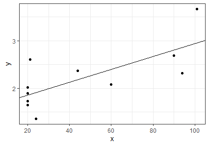
We can graph the Chlorella data and add to it the line described by this slope and intercept:
ggplot(data = chlorella, aes(x = x, y = y)) +
  geom_point() +
  geom_abline(intercept = b[1], slope = b[2]) +
  theme_bw()

Verification

We can verify our results by comparing them with the coefficients produced from the lm() (linear model) function:
lm(y ~ x, data = chlorella)

In this formula, the ~ means ‘as a function of’; here, we fit y as a function of x.  The 1’s that are multiplied by the intercept are automatically accounted for when using lm() and related functions.

The coefficients are labelled differently here, but the values are identical to those that we calculated above.

Call:
lm(formula = y ~ x, data = chlorella)

Coefficients:
(Intercept)            x  
    1.58095      0.01362 

Extensions

Matrix algebra can also be used to calculate other types of information that can be extracted from a regression.  Let’s walk through a few.

Predicted Values of y

The predicted value of y for each observation (row) is the value obtained by applying the coefficients obtained above to that observation’s value of x.  In other words, this is the solution to the linear regression formula that we re-arranged above, Y = Xb:
chlorella$y_pred <- X %*% b

For verification, multiply a value of x times the slope, and add the intercept.

Residuals

The residual for each observation (row) is the difference between the actual and predicted values of y:
chlorella <- chlorella |>
  mutate(resid = y - y_pred)

For verification, see resid(lm(y ~ x, data = chlorella)).

Predicted Values for a Range of x Values

The predicted values across a range of x values simply requires that we specify which values of x we want to use.  Let’s use 50 values that span the range of x in our data:
X_range <- seq(from = min(chlorella$x), to = max(chlorella$x), length.out = 50) |>
  data.frame() |>
  rename(light = 1) |>
  mutate(int = 1) |>
  relocate(int) |>
  as.matrix()

We can now postmultiply X_range by b:

y_range <- X_range %*% b

These could be the values that are graphed as a fit line in ggplot, for example (you can do so and compare to the above graph to verify).

Note that it isn’t necessary to use this many values when graphing a linear fit, but a large number of values would be helpful if we had transformed one of our variables and were back-transforming the fit for presentation – more values will show a smoother curve for the resulting non-linear fit.

Concluding Thoughts

The appeal of this matrix formulation of a linear regression is that it can be easily generalized to any number of explanatory variables – fitting a response as a function of two variables simply adds one column to X and one value to b, but does not change the matrix form of the equation, or the corresponding calculation.  This gives the matrix formulation of this equation incredible flexibility.

References

Ellner, S.P., and J. Guckenheimer. 2021. An Introduction to R for Dynamic Models in Biology. Cornell University, Ithaca, NY.

Gotelli, N.J., and A.M. Ellison. 2004. A Primer of Ecological Statistics. Sinauer Associates, Sunderland, MA.

References

Ellner, S.P., and J. Guckenheimer. 2011. An introduction to R for dynamic models in biology. http://www.cam.cornell.edu/~dmb/DynamicModelsLabsInR.pdf