
Group Comparisons
18 Mantel Test
Learning Objectives
To understand the theory behind Mantel tests.
To apply Mantel tests manually and through R.
Resources
van Mantgem & Schwilk (2009)
Key Packages
require(vegan)
Theory
Mantel (1967) first described this test and used it to examine spatial patterns in the occurrence of leukemia.
The Mantel test examines the correlation between two distance matrices from the same samples. The distance matrices can be based on actual data (species abundances, environmental measurements, spatial coordinates) or hypothesized data (e.g., dummy variables coding for treatments). For example, Mantel tests are commonly used to test for spatial autocorrelation as described below.
Mantel tests assume that the matrices are independent and that the correlations are linear. Of course, since the matrices are being compared to one another, it is also essential that samples are listed in the same order in both matrices.
Mantel tests are generally used in two ways in community ecology:
- To compare two independent empirical matrices. For example, spatial autocorrelation can be explored by comparing a distance matrix based on some response with a distance matrix based on the Euclidean distance between the sample units as determined from their spatial coordinates.
- To assess the goodness of fit between data and an a priori model (i.e., one not generated by this dataset). This is how a Mantel test is used to compare a priori groups. In this case, the second distance matrix is based on hypothesized data about the sample units (e.g., dummy variables coding for treatments). In fact, the generalized ANOSIM statistic from the last chapter is an example of this, but with ranked distances.
See Manly & Navarro Alberto (2017, section 5.6), McCune & Grace (2002, chapter 27) and Legendre & Legendre (2012, section 10.5.1) for more details and examples. Legendre & Legendre (2012) emphasize that Mantel tests should be used to test hypotheses about distances, not about the original variables.
Mantel tests can also be extended to examine the correlation between two matrices while controlling for the effect of a third. This is called a partial Mantel test, and is discussed by Legendre & Legendre (2012, section 10.5.2) and Goslee & Urban (2007). Be aware, however, that support for this is not universal: see Guillot & Rousett (2013) for details.
Legendre et al. (2015) argue that Mantel tests should not be used to detect or control for spatial correlation, and several recent articles have proposed new or alternative approaches to deal with this issue (Lisboa et al. 2014; Crabot et al. 2019).
van Mantgem & Schwilk (2009) used Mantel tests to test for spatial autocorrelation in fire effects. Recent ecological examples include Sun et al. (2019), who compared soil fungal assemblages beneath different shrubs, and Yu et al (2018), who compared geographic and genetic distances among eight populations of a tropical tree.
Key Takeaways
A Mantel test is simply the correlation between two distance matrices obtained from the same sample units. These are often either based on two categories of data or one category of data and a matrix coding an experimental design.
The test statistic ranges from -1 (the two sets of distances are negatively correlated) to +1 (the two sets of distances are positively correlated).
Basic Procedure
The basic procedure for a Mantel test is as follows.
- Convert each data matrix to a dissimilarity matrix. Use an appropriate distance measure for each matrix; the measures do not have to be the same.
- Calculate the correlation between the two dissimilarity matrices. This is the test statistic. As a correlation, this always ranges between -1 and +1.
- Assess statistical significance via a permutation test:
- Shuffle the row and column identities of one dissimilarity matrix, permuting row and column identities together so that matrix symmetry is preserved. For example, if row A is moved down four positions, column A is also moved to the right four positions. Equivalently (and easier to describe), permute the rows of one of the original data matrices and then recalculate the dissimilarity matrix.
- Recalculate the correlation between the two dissimilarity matrices. Save this value.
- Re-shuffle and recalculate the specified number of times. The permutations produce a sampling distribution of correlation values against which the actual test statistic is compared.
- Calculate the P-value as the proportion of permutations that yielded equal or stronger correlations than the actual data did. Note that Mantel tests generally result in a one-tailed test, as in this case. A two-tailed test would be used if we had no a priori suspicion about whether the correlation would be positive or negative. To obtain the P-value for a two-tailed test, we would calculate the proportion of permutations whose correlation coefficient (in absolute value) was greater than the test statistic.
Simple Example, Worked By Hand
We’ll start with the dissimilarity matrix based on the two response variables:
Resp.dist <- dist(perm.eg[ , c("Resp1", "Resp2")])
| Plot1 | Plot2 | Plot3 | Plot4 | Plot5 | |
| Plot2 | 2.828 | ||||
| Plot3 | 4.123 | 2.236 | |||
| Plot4 | 11.314 | 11.662 | 9.849 | ||
| Plot5 | 9.849 | 9.220 | 7.071 | 4.123 | |
| Plot6 | 12.207 | 12.042 | 10.000 | 2.236 | 3.162 |
For clarity, distances between plots from different groups are shown in bold.
We also need to calculate a distance matrix based on our grouping variable (A, B). This variable is of class ‘character’, so we need to change it to class numeric before we can calculate a distance matrix from it. Somewhat confusingly, you need to convert it to a factor before you can express the levels of the factor numerically. Euclidean distances are used to express differences among levels in a factor.
Group.dist <- as.numeric(as.factor(perm.eg$Group)) |>

dist()
| Plot1 | Plot2 | Plot3 | Plot4 | Plot5 | |
| Plot2 | 0 | ||||
| Plot3 | 0 | 0 | |||
| Plot4 | 1 | 1 | 1 | ||
| Plot5 | 1 | 1 | 1 | 0 | |
| Plot6 | 1 | 1 | 1 | 0 | 0 |
The grouping variable is now expressed as a ‘0’ if the plots are in the same group and a ‘1’ if they are in different groups. For clarity, distances between plots from different groups are also shown in bold.
We could examine the correlation between these two distance matrices directly, but it’s easier to track the data if we first combine them into a single object. To convert each distance matrix to a vector, we need to change it to class numeric. We will save these to a new dataframe, naming each column as we create it.
mantel.eg <- data.frame(

Resp = Resp.dist,

Group = Group.dist

)
Look at this object to ensure that you understand it.
The test statistic is the simple correlation between the two columns of values:
with(mantel.eg, cor(Resp, Group))
[1] 0.9390683As with other tests, the significance of this statistic is assessed with a permutation test (not shown here).
Implementation in R (vegan::mantel())
You could easily implement the steps in a Mantel test using functions such as cor(), sample(), etc. Of course, you could also use an existing function. For example, mantel() functions are available in the vegan and ecodist packages. Note that these two functions have the same name, which can cause problems if both packages are open simultaneously.
We’ll use the mantel() function in the vegan package. The usage of this function is:
mantel(

xdis,

ydis,

method = "pearson",

permutations = 999,

strata = NULL,

na.rm = FALSE,

parallel = getOption("mc.cores")

)
The arguments are:
xdis– the first of two dissimilarity matrices to be testedydis– the second of two dissimilarity matrices to be testedmethod– the correlation method ("pearson","spearman", or"kendall") to be applied. The Pearson product-moment correlation is the default. Spearman and Kendall are non-parametric correlations based on the ranks of the distances.permutations– number of permutations to conduct to assess the significance of the correlation, or a list of permutation instructions obtained using thehow()function. This latter option is necessary with complex designs where permutations need to be restricted – we’ll discuss this in a few classes. Default is to conduct 999 permutations without any restrictions to the permutations.strata– integer vector or factor identifying strata that permutations are to be restricted within.na.rm– remove missing observations? Default is no (FALSE)parallel– option for parallel processing.
The results of the Mantel test are saved in an object of class ‘mantel’. This class of object does not currently have summary() or plot() functions associated with it. However, you can explore the object in more detail using the str() function.
The vegan package also includes a mantel.partial() function.
Simple Example
Here, we’ll call the two distance matrices that we created above:
simple.results.mantel <- mantel(

xdis = Resp.dist,

ydis = Group.dist,

method = "pearson",

permutations = 999

)
simple.results.mantel
Mantel statistic based on Pearson's product-moment correlation
Call:
mantel(xdis = Resp.dist, ydis = Group.dist, method = "pearson",
permutations = 999)
Mantel statistic r: 0.9391
Significance: 0.1
Upper quantiles of permutations (null model):
90% 95% 97.5% 99%
0.0283 0.9391 0.9391 0.9391
Permutation: free
Number of permutations: 719
Grazing Example
The script for loading the oak data included calculation of the Bray-Curtis distance matrix based on the compositional data. To conduct a Mantel test, we also need a distance matrix expressing the differences in grazing status:
graz.dist <- as.numeric(as.factor(grazing)) |>

dist()
Now we can compare the two distance matrices:
grazing.results.mantel <- mantel(

xdis = Oak1.dist,

ydis = graz.dist,

method = "pearson",

permutations = 999

)
grazing.results.mantel
We included the default correlation method and number of permutations for completeness. If we were ok with the defaults, we could omit those arguments.
Mantel statistic based on Pearson's product-moment correlation
Call:
mantel(xdis = Oak1.dist, ydis = graz.dist, method = "pearson",
permutations = 999)
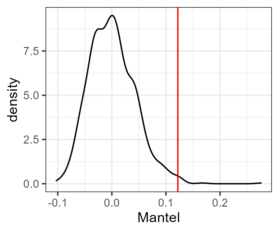
Mantel statistic r: 0.122
Significance: 0.009
Upper quantiles of permutations (null model):
90% 95% 97.5% 99%
0.0555 0.0815 0.1014 0.1144
Permutation: free
Number of permutations: 999
Note, as for all other permutation tests, that the P-value differs slightly among individual runs of this test due to differences among permutations. However, the correlation itself is not affected by the number or identity of the permutations.
Using the str() function, can you figure out how I created this graph of the actual correlation and the distribution of correlations obtained from permutations?
References
Crabot, J., S. Clappe, S. Dray, and T. Datry. 2019. Testing the Mantel statistic with a spatially-constrained permutation procedure. Methods in Ecology and Evolution 10:532-540.
Goslee, S.C., and D.L. Urban. 2007. The ecodist package for dissimilarity-based analysis of ecological data. Journal of Statistical Software 22(7):1-19.
Guillot, G., and F. Rousett. 2013. Dismantling the Mantel tests. Methods in Ecology and Evolution 4:336-344.
Legendre, P., and L. Legendre. 2012. Numerical ecology. 3rd English edition. Elsevier, Amsterdam, The Netherlands.
Legendre, P., M-J. Fortin, and D. Borcard. 2015. Should the Mantel test be used in spatial analysis? Methods in Ecology and Evolution 6:1239-1247.
Lisboa, F.J.G., P.R. Peres-Neto, G.M. Chaer, E.d.C. Jesus, R.J. Mitchell, S.J. Chapman, and R.L.L. Berbara. 2014. Much beyond Mantel: bringing Procrustes Association Metric to the plant and soil ecologist’s toolbox. PLoS ONE 9(6): e101238. doi:10.1371/journal.pone.0101238
Manly, B.F.J., and J.A. Navarro Alberto. 2017. Multivariate statistical methods: a primer. Fourth edition. CRC Press, Boca Raton, FL.
Mantel, N. 1967. The detection of disease clustering and a generalized regression approach. Cancer Research 27:209-220.
McCune, B., and J.B. Grace. 2002. Analysis of ecological communities. MjM Software Design, Gleneden Beach, OR.
Sun, Y., Y. Zhang, W. Feng, S. Qin, and Z. Liu. 2019. Revegetated shrub species recruit different soil fungal assemblages in a desert ecosystem. Plant and Soil 435:81-93.
van Mantgem, P.J., and D.W. Schwilk. 2009. Negligible influence of spatial autocorrelation in the assessment of fire effects in a mixed conifer forest. Fire Ecology 5:116-125.
Yu, N., J. Yuan, G. Yin, J. Yang, R. Li, and W. Zou. 2018. Genetic diversity and structure among natural populations of Mytilaria laosensis (Hamamelidaceae) revealed by microsatellite markers. Silvae Genetica 67:93-98.
Media Attributions
- Mantel
