
Foundational Concepts
5 Data Adjustments
Learning Objectives
To present ways to identify data entry errors.
To consider when and how to script temporary data adjustments.
To begin considering how data adjustments relate to the research questions being addressed.
To continue using R, including functions to adjust data.
Readings
Broman & Woo (2018)
Key Packages
require(tidyverse, labdsv)
Properties of Multivariate Ecological Data
Many ecological studies collect data about multiple variables on the same sample units. Manly & Navarro Alberto (2017, ch. 1) provide several examples of multivariate datasets. Types of data that have been the foci of analyses in this course include:
- Physiology: gas exchange, photosynthesis, respiration, stomatal conductance
- Plant ecology: abundances of multiple species
- Fire ecology: tree mortality, scorch height, fuel consumption, maximum temperature
- Remote sensing: height of LiDAR returns, canopy density, rumple
- Anatomy: morphometric measurements
- Bioinformatics / genomics: genetic sequence data
Since these data are collected on the same units, they are multivariate. However, they often have many properties that confound conventional multivariate analyses:
- Bulky – large number of elements in a matrix
- Intercorrelated / redundant – for example, species often respond to the same gradients, and LiDAR-derived metrics may be highly correlated with one another
- Outliers – non-normal distributions. For example, species composition data is notorious for having lots of zeroes (i.e., species absent from plots)
Given these properties, it is often necessary to adjust data prior to analysis. McCune (2011) provides a decision tree that summarizes multiple options for data adjustment and for analyses. Other suggestions are provided in an appendix to these notes.
Data Organization (redux)
As discussed in the context of reproducible research, scripting is a powerful ability that distinguishes R from point-and-click statistical software. When a script is clearly written, it is easy to re-run an analysis as desired – for example, after a data entry error is fixed or on a particular subset of the data.
Once your data have been entered and corrected, all subsequent steps should be automated in a script. This often requires data manipulation, such as combining data from various subplots, or calculating averages across levels of a factor. New R users often want to export their data to Excel, manipulate it there, and re-import it into R. Resist this urge. Working in R helps you avoid errors that can creep in in Excel – such as calculating an average over the wrong range of cells– and that are extremely difficult to detect. If tempted to export your data file to Excel so that you can re-organize or summarize it, I encourage you to first check out the R help files (including on-line resources), ask colleagues how they solve similar issues, and consult resources like Wickham & Grolemund (2017). Packages like dplyr and tidyr are particularly helpful for these types of tasks.
The general principle is to maintain a single master data file. Obvious errors should be permanently corrected in this master data file, but other changes may be context dependent. Scripting these context-dependent changes enables you to:
- work from the same raw data every time
- avoid having multiple versions of your data file
Broman & Woo (2018) provide many valuable suggestions for organizing data within spreadsheets.
By convention, multivariate data are organized in a matrix where each row is a unique sample unit and each column is a unique variable. This is consistent with the ‘tidy data’ philosophy within the tidyverse:
- Each variable is its own column. I often refer to the columns as ‘species’ for simplicity, but they might be measured values or assigned values such as plot ID, year, experimental treatment etc.
- Each sample unit is its own row. I often refer to the rows as ‘plots’ for simplicity, but they might be stands or plot-year combinations (i.e., a measurement of a given plot at a point in time) or other units of observation. The units will depend on the study system, but it is essential that each row be uniquely identified.
This structure for organizing data is called the ‘wide’ format in tidyr. In practice, data are sometimes stored in a ‘long’ or triplet form where one column identifies the sample unit, one column identifies the variable, and one column identifies the value of that variable in that sample unit. These organizational structures are related, as illustrated in the below figure.
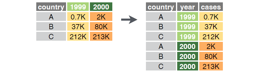
The tidyr package includes the pivot_wider() function to convert data from long to wide format, and the pivot_longer() function to convert from wide to long format.
Triplet form can be a particularly efficient way to store compositional data as many species are often absent from most sample units. If all non-zero values are included in the triplet form, the zeroes can be inferred and automatically added when data are converted to wide format.
Data Organization
Store data in master data files, with sample units as rows and variables as columns. Each row should have a unique identifier, and each column should contain a single variable.
Describe the rows and columns of the master data file in a metadata document.
Ideally, prepare a single master data file for data collected at each spatial scale. Apply unique identifiers consistently across data files so they can be merged within R.
Identify and Permanently Correct Data Entry Errors
I am assuming here that the data we are using are organized in one or more spreadsheets; Broman & Woo (2018) provide valuable ideas on how to do so.
It may seem self-evident, but it’s important to check for and correct data errors before proceeding to analysis. Data cleaning can be more time-consuming than the actual analyses that follow (de Jonge & van der Loo 2013). Although I rely exclusively on R once I’m ready for analysis, I generally do this initial type of quality control in Excel (via Pivot Tables, etc.) before importing data into R. However, de Jonge & van der Loo (2013) provide detailed notes about how to explore and clean up data within R. Zuur et al. (2010) provide very helpful suggestions for data exploration.
Ways to identify data entry errors include:
- Recheck the data entry on a randomly selected subset of the data. This can be done by yourself or by having someone read the data back to you.
- Decide how to deal with missing data. See suggestions of McCune & Grace (2002, p. 58-59) and de Jonge & van der Loo (2014, ch. 3).
- Examine the minimum and maximum values to verify that they span the permitted range of values.
- If dealing with a categorical variable, view the unique values recorded and make sure they are all appropriate. Watch out for seemingly minor differences:
- A plot with a topographic position of ‘slope’ will be assigned to a different category than one with a position of ‘Slope‘ (note the capital!).
- Similarly, ‘slope’ and ‘slope ‘ would be treated as two different values because of the space in the latter.
- Plot reasonably correlated variables against one another to identify potential bivariate outliers. These might reflect data entry errors, though they may also be true outliers (see below). Anomalies can also sometimes be detected by calculating the ratio of two variables (e.g., tree height and diameter) and then looking at the extreme values in the distribution of this ratio. This technique is less appropriate for community data than for other types of data (e.g., environmental variables that are correlated with one another).
- If you are dealing with compositional data, resolve unknowns and assign each unknown species to a unique species code. Be sure to keep track of what you’ve done – you may encounter that unknown code again elsewhere! It is often helpful to save two species codes for each entry: one for the original field code, and one for the code to be analyzed.
In spite of our best efforts at quality control, errors sometimes slip through. This is where scripts really shine. If you have kept careful track of the steps in your analysis (see the ‘Reproducible Research’ chapter), once you have corrected these errors you will be able to easily re-do your analyses, re-create graphics, etc. simply by re-running the script.
Related to this is the issue of detecting outliers. Univariate outliers are relatively easy to detect. However, we have already noted that community ecology data are often non-normally distributed – in particular, there is usually a plethora of zeros (absences) in a site × species matrix. These might appear to be outliers statistically, but they aren’t outliers biologically and shouldn’t be treated as such!
Multivariate outliers are much more difficult to detect. One way to do so is to compare the range of dissimilarities among elements. See here for more detail.
An interesting non-R option for cleaning up messy data is OpenRefine (https://openrefine.org/). I have not used this website, however, so cannot speak to its effectiveness.
Scripted (Temporary) Data Adjustments
Often we may want to adjust the data for an analysis but do not want to permanently change the original data file. We will consider three types of temporary adjustments here: consolidating taxonomy, deleting sample units, and deleting rare species. These types of adjustments are often required for compositional analyses but may be less common for other types of multivariate data.
Scripted Adjustments to Data
Scripts provide a means of adjusting the data for an analysis without permanently changing the original data file. Examples of these adjustments include:
- Consolidating taxonomy
- Deleting sample units (rows) – either because they are empty or to focus on a subset of them
- Deleting species (columns) because they are absent from the focal sample units or are rare and assumed to contribute little to the patterns among sample units
Your analytical methods should clearly identify whether and which adjustments were made.
Consolidating Taxonomy
It can be difficult to identify the taxa present in an ecological study, and people vary in their taxonomic proficiency. In one study (Morrison et al. 2020), more than half of the apparent differences in cover of plant species over time were identified as observer errors! As another example, I analyzed compositional variation in grasslands around the world (Bakker et al. 2023). Each site has multiple plots, and each plot was assessed in multiple years. As part of my quality control, I reviewed which species were identified within each site and year and highlighted inconsistencies that likely reflect the person doing the work (as in the example below) rather than actual ecological changes. My analysis includes scripted adjustments to taxonomy at 70% of the 60 sites in the analysis, indicating that this is not a rare scenario.
Consider the following example of species composition in two plots in two years:
| Year | Plot | Poa compressa | Poa pratensis | Poa spp. |
| 1 | i | 1 | 3 | |
| 1 | ii | 2 | 2 | |
| 2 | i | 4 | ||
| 2 | ii | 4 |
This might happen, for example, if the person who assessed composition in year 2 was less confident in their ability to distinguish the two Poa spp. than the person who assessed composition in year 1.
Analyses that focus just on Year 1 would likely want to include the fact that two species of Poa were documented that year. For example, these species might respond differently to environmental conditions or to experimental factors.
What about comparisons between Years 1 and 2? As reported here, each plot has lost two species (Poa compressa and P. pratensis were present in Year 1 but absent in Year 2) and gained one species (Poa spp.). However, it should be clear that these are differences in taxonomic resolution rather than meaningful ecological changes. Instead, it would be reasonable to combine P. compressa and P. pratensis for analyses that compare the years. This can be easily scripted:
- Add the covers of P. compressa, P. pratensis, and Poa spp., and assign the summed cover to a column with a new taxonomic code, such as ‘Poa_combined’.
- Delete the columns for P. compressa, P. pratensis, and Poa spp.
To run this in R, we’ll first create our dataset and then use the mutate() function from the tidyverse. Of course, there are many other ways that this could also be scripted.
poa_example <- data.frame(
Year = c(1, 1, 2, 2),
Plot = c("i", "i", "ii", "ii"),
Poa_compressa = c(1, 2, 0, 0),
Poa_pratensis = c(3, 2, 0, 0),
Poa_spp = c(0, 0, 4, 4))
library(tidyverse)
poa_adjusted <- poa_example %>%
mutate(Poa_combined = Poa_pratensis + Poa_compressa + Poa_spp,

.keep = "unused")
  Year Plot Poa_combined
1    1    i            4
2    1    i            4
3    2   ii            4
4    2   ii            4
Note that the abundance of ‘Poa_combined’ is identical in all plots and years of this simple example; this was not obvious from the original data.
Deleting Sample Units (Rows)
With some types of ecological data, it is possible for sample units to be empty – for example, there might be no species growing in a vegetation plot. While this information is ecologically relevant, many analytical techniques require that every row of the matrix contain at least one non-zero value. There are two common ways to deal with empty sample units:
- Delete empty sample units from the analysis. This is not ideal for several reasons:
- It reduces the size of the dataset and can alter the balance of our design.
- It changes the questions being asked. For example, imagine that we assessed plots in two habitats, and that many of the sample units in one of the habitats were empty. Using all of the sample units, we can ask whether composition differs between habitats. Using only those sample units that contain species, we can ask whether composition differs between habitats given that we are only considering areas that contain species.
- Add a dummy variable with a small value to all sample units (Clarke et al. 2006). Doing so means that all sample units have at least one non-zero variable, permitting their inclusion in analyses that require data in all rows. I’ll illustrate this approach in the chapter about distance measures.
If data are stored in multiple objects, such as when response variables are in one object and potential explanatory variables are in another, we need to apply changes to both objects. If we delete a sample unit (row) from one object, we also need to remove that sample unit from the other object. And, of course we need to make sure that the remaining sample units are in the same order in both objects.
Another reason to delete sample units is to focus on a subset of the data for a particular analysis. The filter() function from the tidyverse is very useful here. For example, if we wanted to focus on Year 1 from poa_example above:
poa_example %>% filter(Year == 1)
  Year Plot Poa_pratensis Poa_compressa Poa_spp
1    1    i             1             3       0
2    1    i             2             2       0
Deleting Species (Columns)
Sometimes a dataset includes columns that are empty. For example, this often happens with compositional data if you’ve filtered the data to focus on a subset of the sample units; some species were never recorded in the subset that you’re focusing on. These ‘empty’ species are less of a computational concern than empty sample units, though relativizations that are applied to columns (see ‘Relativizations‘ chapter) can produce ‘NaN’ values if applied to empty columns. It is also computationally inefficient to include a large number of empty columns, though computing power is no longer a significant consideration for most analyses. We can delete these empty columns before proceeding with analyses.
A more intriguing instance can arise with compositional data: some people suggest that we delete rare species. It may seem counter-intuitive to ignore these species, but the logic is that rare species are often poorly sampled and therefore contribute little information about the relationship with environmental gradients, etc. (I suspect that concerns about computing power were also a factor in developing this recommendation, but are no longer relevant).
When is a species rare? A cutoff of 5% of sample units is often adopted. So, if a dataset contains 20 sample units, the 5% rule indicates that species that only occur in a single sample unit should be deleted. If a dataset contains 40 sample units, species that occur in one or two sample units would be deleted.
When data have been collected in distinct areas (e.g., experimental treatments), deletion could occur on the basis of the full dataset (i.e., species that occur on < 5% of all sample units) or on individual treatments (i.e., species that occur on < 5% of the sample units in a given treatment). Generally, however, sample sizes are too low for the latter approach to be meaningful.
Surprisingly few studies have examined the effect of removing rare species. Cao et al. (2001) noted that consideration of the dominant species often provides insight into major environmental gradients, and concluded that “the theoretical or empirical justification for deleting rare species in bioassessment is weak”. Poos & Jackson (2012) used electrofishing to sample the fish community at each of 75 sites in a watershed. They analyzed these data after making four types of adjustments: i) using the full dataset (no species removed), ii) removing species occurring at a single site, iii) removing those occurring at less than 5% of sites, and iv) removing those occurring at less than 10% of sites. The effect of these removals was compared with the effects of choice of distance measure and choice of ordination method, both of which we’ll discuss later. They concluded that removal of rare species had about as large an effect on the conclusions as did the choice of ordination method. Brasil et al. (2020) examined how the compositional variation within fish and insect communities was affected by systematically removing rare or common species (though they defined rarity by abundance rather than by the number of sample units in which a species was present). They concluded that the proportion of compositional variation that could not be explained by their explanatory variables – aka the residual variation – was minimally affected even by the removal of half of the species. This was especially true if variation was expressed on the basis of abundance rather than presence. Further examination of this topic is clearly warranted (anyone want to include this in their project?). As a counter to this focus on rare species, Avolio et al. (2019) provide a nice consideration of the importance and identification of dominant species.
There is no requirement that rare species be removed from a community ecology study; it is up to you to decide whether to do so or not. Of course, you should clearly state whether you did, why, and what your minimum rarity threshold was.
Please note that the above considerations are not applicable in all circumstances. Rarity in this context refers to sample units where a species was not detected. If your response variables are not species, then your data may contain values for all sample units. And, even if there are some rare ‘species’, it may not make sense to remove them. For example, if your response variables were measures of burn severity, it likely would make sense to retain all burn severities even if they were not detected in your particular study.
Finally, bioinformatics studies include pipelines that include pre-processing steps which can effectively remove species from a dataset, particularly for speciose systems such as microbial systems (Zhan et al. 2014).
Application in R
Rare species (response variables; columns) can be removed manually, but it is easier to use an existing function. We’ll illustrate this using our sample dataset.
After opening your R project, load the sample dataset:
Oak <- read.csv("data/Oak_data_47x216.csv", header = TRUE, row.names = 1)
Oak_species <- read.csv("data/Oak_species_189x5.csv", header = TRUE)
Create separate objects for the response and explanatory data:
Oak_abund <- Oak[ , colnames(Oak) %in% Oak_species$SpeciesCode]
Oak_explan <- Oak[ , ! colnames(Oak) %in% Oak_species$SpeciesCode]
See the ‘Loading Data‘ chapter if you do not understand what these actions accomplished.
Oak_abund contains species abundance data for 189 species encountered on the 47 stands. Therefore, a 5% cutoff (47 x 0.05 = 2.35) means deleting species that occur in less than 3 stands.
labdsv::vegtab()
This function eliminates rare species and re-orders the columns and/or rows in a data frame. The help file for this function shows its usage:
vegtab(comm, set, minval = 1, pltord, spcord, pltlbl, trans = FALSE)
The key arguments are:
comm– the data frame containing the data to be analyzedminval– the minimum number of observations that a variable has to occur to be retained. The default is 1 observation (i.e., empty variables – those without any occurrences – are deleted)pltord– a numeric vector specifying the order of rows in the outputspcord– a numeric vector specifying the order of columns in the output
To use this function, we need to specify the dataframe (comm argument) and the minimum number of observations (minval argument). Since we are not seeking to re-order our dataframe, we do not need to specify the pltord or spcord arguments.
Oak_no_raw <- vegtab(comm = Oak_abund, minval = (0.05 * nrow(Oak_abund)))
Note how I set minval equal to 5% of the number of samples, without specifying how many samples there were. This approach provides flexibility as it remains correct even if the number of rows in the dataset changes. If I didn’t need this flexibility, I could equivalently have hard-coded the minimum number of observations (minval = 3).
How many species are in the reduced dataset? ______
How many species were in the original dataset? _______
How many species were removed? _____
For clarity, I named each argument explicitly in the above code. If we list the arguments in the order specified by a function’s usage, we can omit the argument names. Or, we can just use a smaller unique portion of the argument name and let R match it against the arguments to figure out which one we mean:
Oak_no_raw <- vegtab(Oak_abund, min = (0.05 * nrow(Oak_abund)))
While these usages are more compact, they can be frustrating if you have to figure out later which arguments are being used. I specify arguments by name to avoid this.
Once you’ve removed rare species, you may have to check again for empty sample units.
Concluding Thoughts
Decisions about how to adjust data – including whether to consolidate taxonomy, focus on a subset of the sample units, and to delete rare species – can strongly affect the conclusions of subsequent analyses.
Empty sample units and rare species should never be deleted when analyzing species richness or diversity. In these calculations, the rare species are of critical importance, and a sample unit containing no species will affect the mean species richness, the slope of a species-area curve, etc. This is another reason to script these adjustments and preserve the original data.
References
Avolio, M.L., E.J. Forrestel, C.C. Chang, K.J. La Pierre, K.T. Burghardt, and M.D. Smith. 2019. Demystifying dominant species. New Phytologist 223:1106-1126.
Bakker, J.D., J.N. Price, J.A. Henning, E.E. Batzer, T.J. Ohlert, C.E. Wainwright, P.B. Adler, J. Alberti, C.A. Arnillas, L.A. Biederman, E.T. Borer, L.A. Brudvig, Y.M. Buckley, M.N. Bugalho, M.W. Cadotte, M.C. Caldeira, J.A. Catford, Q. Chen, M.J. Crawley, P. Daleo, C.R. Dickman, I. Donohue, M.E. DuPre, A. Ebeling, N. Eisenhauer, P.A. Fay, D.S. Gruner, S. Haider, Y. Hautier, A. Jentsch, K. Kirkman, J.M.H. Knops, L.S. Lannes, A.S. MacDougall, R.L. McCulley, R.M. Mitchell, J.L. Moore, J.W. Morgan, B. Mortensen, H. Olde Venterink, P.L. Peri, S.A. Power, S.M. Prober, C. Roscher, M. Sankaran, E.W. Seabloom, M.D. Smith, C. Stevens, L.L. Sullivan, M. Tedder, G.F. Veen, R. Virtanen, and G.M. Wardle. 2023. Compositional variation in grassland plant communities. Ecosphere 14(6):e4542. https://doi.org/10.1002/ecs2.4542.
Brasil, L.S., T.B. Vieira, A.F.A. Andrade, R.C. Bastos, L.F.d.A. Montag, and L. Juen. 2020. The importance of common and the irrelevance of rare species for partition the variation of community matrix: implications for sampling and conservation. Scientific Reports 10:1977. Doi: 10.1038/s41598-020-76833-5
Broman, K.W., and K.H. Woo. 2018. Data organization in spreadsheets. The American Statistician 72:2-10. Doi:10.1080/00031305.2017.1375989
Cao, Y., D.P. Larsen, and R.St-J. Thorne. 2001. Rare species in multivariate analysis for bioassessment: some considerations. Journal of the North American Benthological Society 20:144-153.
Clarke, K.R., P.J. Somerfield, and M.G. Chapman. 2006. On resemblance measures for ecological studies, including taxonomic dissimilarities and a zero-adjusted Bray-Curtis coefficient for denuded assemblages. Journal of Experimental Marine Biology and Ecology 330:55-80.
de Jonge, E., and M. van der Loo. 2013. An introduction to data cleaning with R. Statistics Netherlands, The Hague, Netherlands. 53 p. http://cran.r-project.org/doc/contrib/de_Jonge+van_der_Loo-Introduction_to_data_cleaning_with_R.pdf
Manly, B.F.J., and J.A. Navarro Alberto. 2017. Multivariate statistical methods: a primer. Fourth edition. CRC Press, Boca Raton, FL.
McCune, B. 2011. A decision tree for community analysis [poster]. MjM Software Design, Gleneden Beach, OR.
McCune, B., and J.B. Grace. 2002. Analysis of ecological communities. MjM Software Design, Gleneden Beach, OR.
Morrison, L.W., S.A. Leis, and M.D. DeBacker. 2020. Interobserver error in grassland vegetation surveys: sources and implications. Journal of Plant Ecology 13(5):641-648.
Poos, M.S., and D.A. Jackson. 2012. Addressing the removal of rare species in multivariate bioassessments: the impact of methodological choices. Ecological Indicators 18:82-90.
Posit. 2023. Data tidying with tidyr :: cheatsheet. https://rstudio.github.io/cheatsheets/tidyr.pdf
Wickham, H., and G. Grolemund. 2017. R for data science: import, tidy, transform, visualize, and model data. O’Reilly Media, Sebastopol, CA. http://r4ds.had.co.nz/
Zhan, A., W. Xiong, S. He, and H.J. MacIsaac. 2014. Influence of artifact removal on rare species recovery in natural complex communities using high-throughput sequencing. PLoS ONE 9(5):e96928.
Zuur, A.F., E.N. Ieno, and C.S. Elphick. 2010. A protocol for data exploration to avoid common statistical problems. Methods in Ecology and Evolution 1:3-14.
Media Attributions
- long.v.wide.table.format
