
Classification
34 Univariate Regression Trees
Learning Objectives
To understand how a univariate regression tree (URT) uses a set of explanatory variables to split a univariate response into groups.
To understand the importance of the complexity parameter (cp) table in evaluating a URT.
To build and interpret regression trees.
To explore how cross-validation allows assessment of how well a URT can predict the group identity of data that were not part of the tree’s construction.
Readings (Recommended)
De’ath & Fabricius (2000)
Key Packages
require(tidyverse, mvpart, ggdendro)
Introduction
A univariate regression tree (URT) relates a single response variable to one or more explanatory variables. Many other techniques have this same overall goal; the difference for a URT is that:
- The dataset is divided via binary splits into mutually exclusive nodes (groups) such that the observations in each node are as similar as possible with respect to the response variable.
- Different explanatory variables can be used at each split.
The result is a tree structure in which each split divides the dataset into two groups.
Key Takeaways
A univariate regression tree (URT) evaluates multiple explanatory variables and identifies the value of one of those variables that separates sample units into two groups where the variance of a univariate response is minimized in those groups.
This process is then repeated independently for each group. The iterative or hierarchical nature of this process means that initial decisions can have cascading effects throughout the tree.
The URT Process
Groups are identified via binary splits in a tree structure: each split divides the dataset into two groups.
We begin by specifying the response variable and a number of potential explanatory variables. The response data are in a single node, called the root node. Therefore, this is a divisive approach – we seek to split the data into smaller groups.
A suite of potential explanatory variables are evaluated. These variables can be of any type – it is important that each explanatory variable is recognized as the correct class of object. We have seen numerous examples of categorical variables (e.g., male vs. female) and of continuous variables (e.g., elevation), but not many of ordinal variables (e.g., low / medium / high). For ordinal variables, the ordering of the levels is important and needs to be specified correctly so that the relative ordering of the levels is incorporated into the analysis. One way to do so is with the ordered() function. If an ordinal variable is not specified correctly, the tree could distinguish between potentially non-sensical combinations of levels (e.g., medium vs. low or high).
Each potential explanatory variable is compared to the response variable to identify:
- The value of the explanatory variable that would most strongly separate the response data into two nodes, and
- How well that explanatory variable would separate the data.
These decisions are made using the assumption that the goal is to identify nodes that are as homogeneous as possible with respect to the response variable. Homogeneity is assessed by calculating the impurity of the node: a completely homogeneous node contains zero impurity. Impurity can be calculated in different ways, depending on the characteristics of the response variable:
- Continuously-distributed: minimizing the within-node sums of squares (or, equivalently, maximizing the between-node sums of squares)
- Categorical: minimizing the misclassification rate
The explanatory variable that splits the root note into the most homogeneous pair of branches is selected. In other words, splitting on the basis of this variable at this value results in the lowest impurity. Each sample unit is assigned to one of the two nodes based on its value of the explanatory variable.
Now, the key step: each node is treated as an independent subset and the above procedure of comparing explanatory variables and identifying the one that most strongly reduces the impurity of the resulting groups is repeated for each. This process of treating nodes as independent subsets and analyzing them independently is why a URT can yield nonlinear solutions.
All splits are optimal for the node and are evaluated without regard to other splits in the tree or the performance of the whole tree. However, the characteristics of the observations in a given node are conditional on earlier splits in the tree.
Splitting continues until one or more stopping criteria are satisfied. These stopping criteria include:
- A minimum number of observations that a node must contain to be split further. Nodes with fewer than this number of observations are called leaves or terminal nodes.
- A minimum number of observations that a terminal node must contain. For example, it generally would not be helpful to split a node such that a leaf contained a single observation.
- A minimum amount by which a split must increase the overall model fit in order to be performed. This amount is known as the complexity parameter (cp).
Once the tree is grown, it is examined to determine whether it should be pruned back to a smaller and more desired size. The desired tree size can be established many ways, but often involves cross-validation. Cross-validation involves omitting one or more observations from the dataset, building a tree from the rest of the dataset, and then examining how well the tree predicts or classifies the omitted observation. The tree with the smallest predicted mean square error is the “best predictive tree” and should give the most accurate predictions.
The fit of a tree is assessed by calculating the proportion of the total sum of squares that it explains. Trees are summarized by their size (number of leaves) and overall fit (fraction of variance not explained by the tree). Fit can be defined by:
- relative error – total impurity of leaves divided by impurity of root node (i.e., undivided data), or the fraction of the total variance that is not explained by the tree. In other words, 1 – R2. Ranges from 0 to 1. Shown by open circles in Figure 3 (below, from De’ath 2002).
- cross-validated relative error – calculated based on the cross validations. Ranges from 0 (perfect predictor) to ~1 (poor predictor), and is always equal to or higher than that based on the full dataset. Shown by closed circles in Figure 3 below. The horizontal dashed line in the figures is 1 SE above the lowest cross-validated relative error.

For classification trees, the fit of the tree is assessed via misclassification rates. A confusion matrix is generated, where the rows are the observed classes and the columns are the predicted classes. Values along the diagonal are correctly classified while all others are misclassified.
A Worked URT Example
Let’s illustrate the steps in a URT. We’ll focus on one spider species, troc.terr, and one potential explanatory variable, water. See the introductory notes for instructions about loading these data. We’ll do some illustrative computations, not all possible comparisons.
Decisions about how to split the data will be made on the basis of the variance within the resulting groups. We can calculate the total variance using Huygens’ theorem (recall this from the notes about PERMANOVA?): the sum of squared differences between points and their centroid is equal to the sum of the squared interpoint distances divided by the number of points.
Since I’m going to calculate variances for different splits of the data below, I’ll create a function to do so.
calculate.variance <- function(object, value) {
object %>%
mutate(breakpoint = if_else(water < value, "low", "hi")) %>%
group_by(breakpoint) %>%
summarize(N = length(troc.terr),
variance = sum(dist(troc.terr)^2) / N,
mean = mean(troc.terr))
}
Note that this is hard-coded with water as the explanatory variable and troc.terr as the response variable. We specify the name of the object containing these variables and the value of water at which we want to split the data. This function is available in the GitHub repository.
Root Node
Here’s a simple scatterplot of the data.
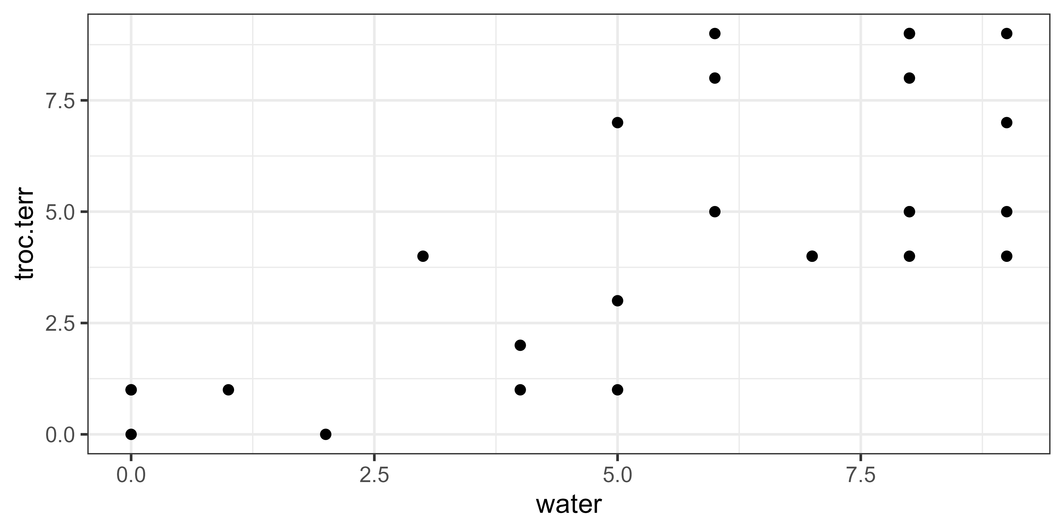
Summarizing the data in the root node:
calculate.variance(object = spider, value = NA)
# A tibble: 1 × 4
  breakpoint     N variance  mean
  <chr>      <int>    <dbl> <dbl>
1 NA            28      263   4.5
The total variance within the dataset is 263, and the average spider abundance is 4.5. Note that this calculation doesn’t depend on the explanatory variable at all.
Identifying First Binary Split
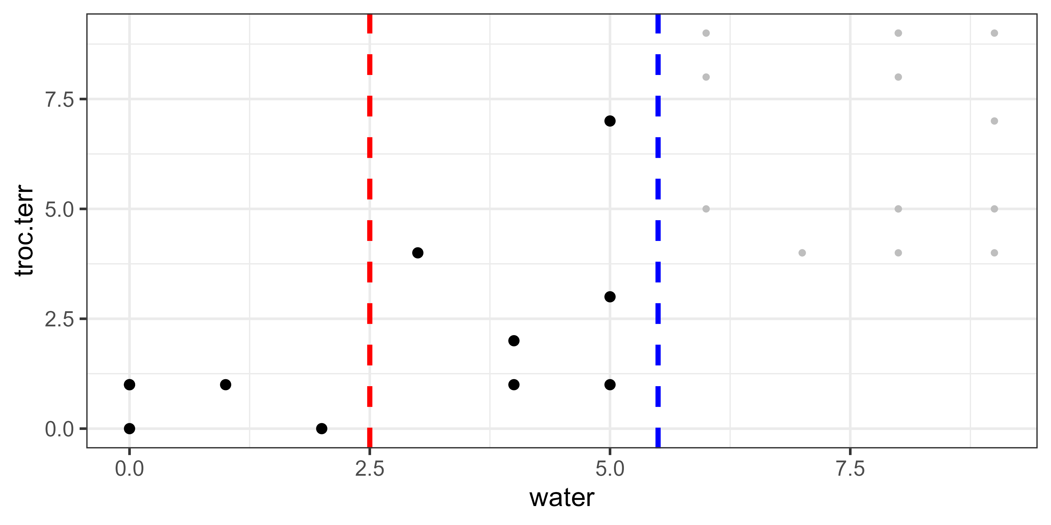
Now, let’s divide the data into two groups on the basis of the explanatory variable. There are many ways we could do so, but any number between two unique values of water will give the same answer – for example, imagine drawing a vertical line below at 2.1 or 2.5 or 2.9. This means we can simply focus on the midpoints between the unique values, shown by the dashed vertical lines here:

Each of these lines would be evaluated separately. For example, the line at water = 2.5 distinguishes sample units with water below this value from sample units above this value:
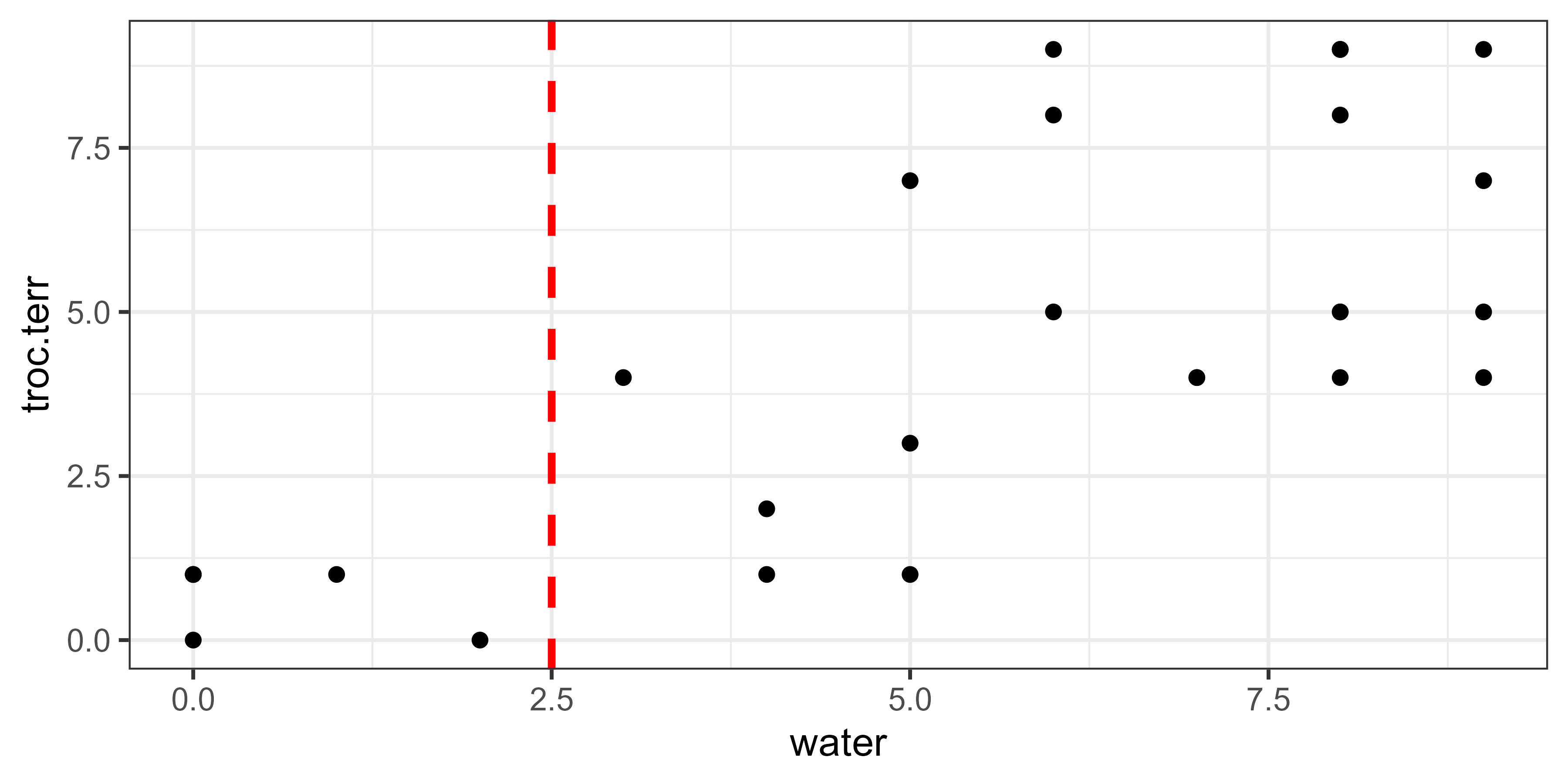
How would this break point affect the variation within the associated groups? We can use Huygens’ theorem again, applying it separately to each group:
calculate.variance(object = spider, value = 2.5)
# A tibble: 2 × 4
  breakpoint     N variance  mean
  <chr>      <int>    <dbl> <dbl>
1 hi            22   149.   5.55
2 low            6     1.33 0.667
The total variance within these groups is 149 + 1.33 = 150.33. The difference between this and the total variance in the dataset (263; see root node above) is the variance between the two groups. There are 22 plots in the ‘hi’ group and they have a mean spider abundance of 5.55. There are 6 plots in the ‘low’ group and they have a mean abundance of 0.67.
Let’s consider a few other break points.
Water = 5.5:
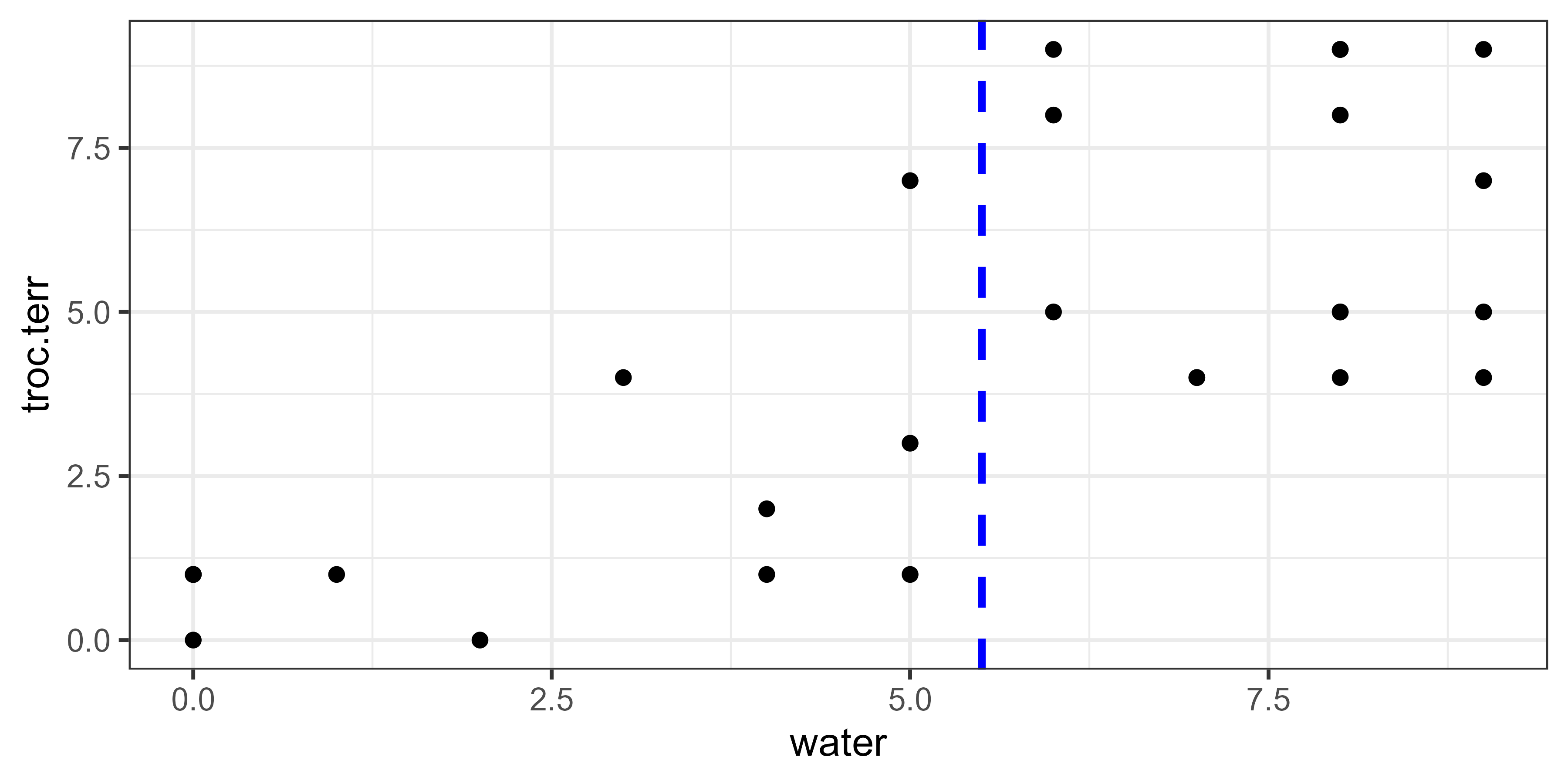
calculate.variance(object = spider, value = 5.5)
# A tibble: 2 × 4
  breakpoint     N variance  mean
  <chr>      <int>    <dbl> <dbl>
1 hi            16     70    6.5
2 low           12     43.7  1.83
Total variance within groups = 70 + 43.7 = 113.7.
Water = 7.5:
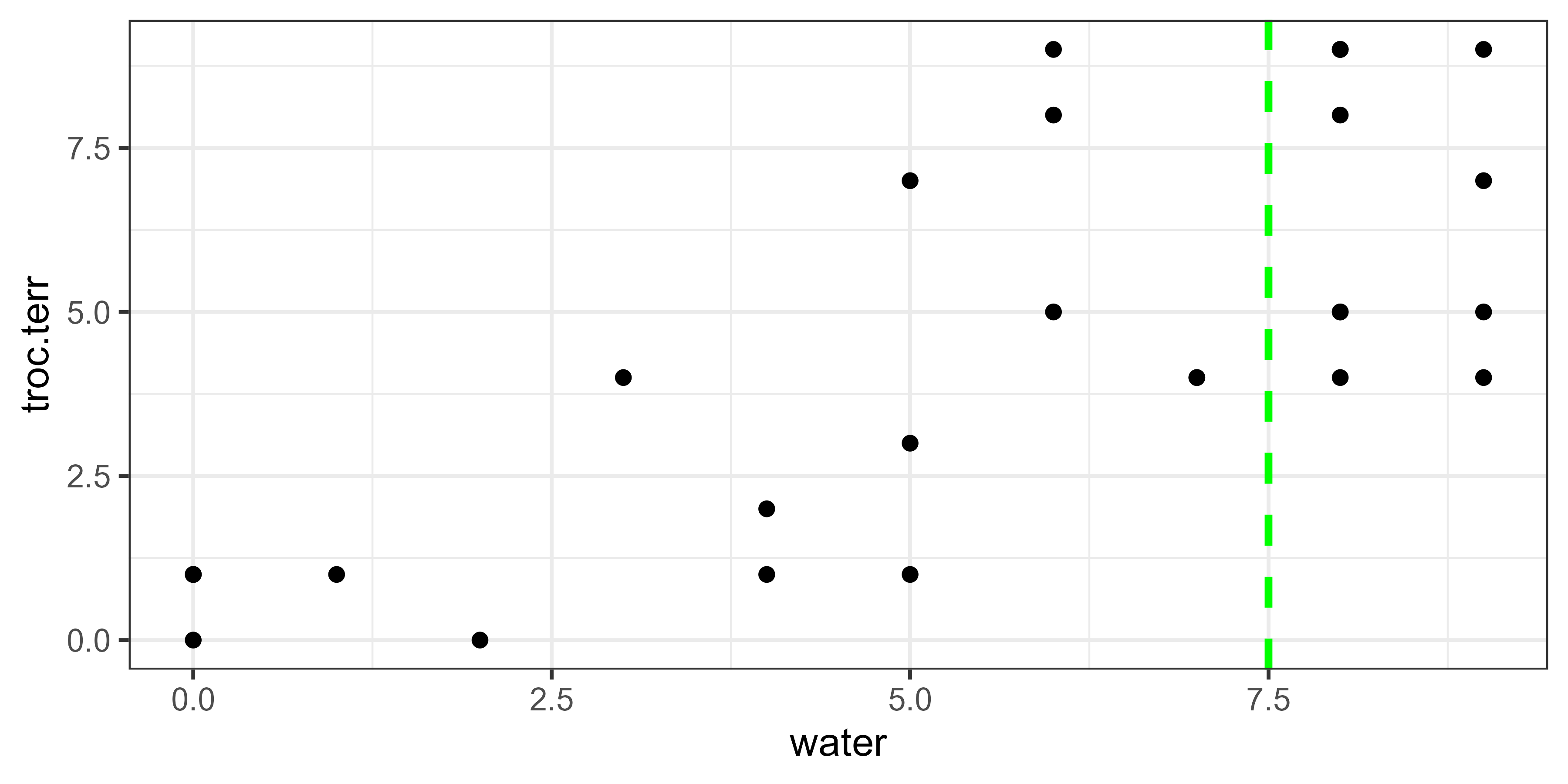
calculate.variance(object = spider, value = 7.5)
# A tibble: 2 × 4
  breakpoint     N variance  mean
  <chr>      <int>    <dbl> <dbl>
1 hi            11     46.2  6.73
2 low           17    127.   3.06
Total variance within groups = 46.2 + 127 = 173.2.
Summarizing this information:
| Break point | Variance Within Groups |
| None (i.e., Total) | 263 |
| water = 2.5 | 150.33 |
| water = 5.5 | 113.7 |
| water = 7.5 | 173.2 |
Of the three potential break points that we calculated, the lowest within-group variance is produced when water = 5.5. Therefore, this is the one that we would use to form the first binary split.
Using this break point, the unexplained variance is 113.7. We can also express this as a proportion of the total variance calculated above: 113.7 / 263 = 0.432. This is the relative error associated with this split.
Note 1: I illustrated this approach by testing three potential splits of water, but operationally a URT will evaluate all possible splits. You can use the R functions below to verify that if water is the only potential explanatory variable specified, the optimal break point is water = 5.5.
Note 2: I illustrated this approach by testing one potential explanatory variable, but operationally a URT will evaluate all specified potential explanatory variables. Whether the split occurs on the basis of water will depend on which other potential explanatory variables are in the model, and how well the optimal splits for those variables minimize impurity within the groups.
Code to create above figures of various break points (comment out lines as desired):
ggplot(data = spider, aes(x = water, y = troc.terr)) +
geom_point() +
geom_vline(xintercept = c(1.5, 2.5, 3.5, 4.5, 5.5, 6.5, 7.5, 8.5),
col = "grey", linetype = "dashed", linewidth = 1) +
geom_vline(xintercept = 2.5, col = "red",

linetype = "dashed", linewidth  = 1) +
geom_vline(xintercept = 5.5, col = "blue",

linetype = "dashed", linewidth = 1) +
geom_vline(xintercept = 7.5, col = "green",

linetype = "dashed", linewidth = 1)+
theme_bw()
Identifying Second Binary Split
Now, the process is repeated with one of the groups created from the above binary split. Let’s start with the group defined by water < 5.5, ignoring observations with water ≥ 5.5. The summary of this split above indicates that there are 12 observations with water < 5.5. How can we most strongly separate these 12 observations into two groups?
Again, all possible splits are evaluated. For illustrative purposes, we’ll just consider one possible split of these data – water = 2.5:
In this graphic, the group of points are to the left of the dashed blue line; the values above this line are shown as small grey points because they are excluded from all calculations with respect to this binary split. The dashed red line is the possible break point at 2.5. Note that this is the same break point that we saw above when considering the first split binary split; the group to the left of this is unchanged but the group to its right now includes fewer values.
spider %>%
filter(water < 5.5) %>%
calculate.variance(value = 2.5)
# A tibble: 2 × 4
  breakpoint     N variance  mean
  <chr>      <int>    <dbl> <dbl>
1 hi             6    26    3
2 low            6     1.33 0.667
The total variance within these groups = 26 + 1.33 = 27.33.
Again, all possible values of the binary split of this group are assessed and the split that produces the smallest within-group variation is identified. If there were multiple potential explanatory variables, they would each be evaluated using this subset of the full dataset.
If we selected this break point to split the data, then the remaining variance within groups would be calculated as the variance within these groups plus the variance within the other group from the first split (water ≥ 5.5; variance = 70; see above). Therefore, the total variance within groups is 26 + 1.33 + 70 = 97.33, and the relative error has decreased to 97.33 / 263 = 0.370.
Code to create above figure:
ggplot(data = spider, aes(x = water, y = troc.terr)) +
geom_point(size = 0.75, colour = "grey") +
geom_point(data = spider[spider$water < 5.5 , ]) +
geom_vline(xintercept = 5.5, col = "blue",

linetype = "dashed", size = 1) +
geom_vline(xintercept = 2.5, col = "red",

linetype = "dashed", size = 1) +
theme_bw()
Identifying Third Binary Split, and Beyond
For the third split, we focus on the data from the group with water ≥ 5.5 and determine which of the possible splits of these data will most strongly separate them into two groups. I haven’t shown this process here; it’s the same as we saw for the second split. Again, the data from the other group (water < 5.5) are not part of this calculation.
This process repeats for all subsequent groups. The process stops when one or more of the stopping criteria are satisfied.
Regression Trees in R
There are several packages that will conduct regression trees in R, including rpart (part of the base installation), mvpart, tree, and party (Hothorn et al. 2006).
We’ll focus on mvpart. See previous chapter for details about how to install mvpart from a github archive.
In addition to the functions used below, mvpart contains several other useful functions, including:
scaler()– various standardization methods.gdist()– calculates dissimilarities. Bray-Curtis distances are the default.xdiss()– calculates ‘extended dissimilarities’ (De’ath 1999). Meant for datasets that span long gradients and therefore contain sample units that do not have species in common. This is comparable to thestepacross()function from vegan.
mvpart::mvpart()
The function we will use is called mvpart(). This function contains lots of arguments because it is a ‘wrapper’ function: it automatically calls several other functions during its execution. In particular, it calls rpart(), the work-horse function that actually does the regression tree, as well as functions to conduct cross-validations, plot the data, etc. Its usage is:
mvpart(form,
data,
minauto = TRUE,
size,
xv = c("1se", "min", "pick", "none"),
xval = 10,
xvmult = 0,
xvse = 1,
snip = FALSE,
plot.add = TRUE,
text.add = TRUE,
digits = 3,
margin = 0,
uniform = FALSE,
which = 4,
pretty = TRUE,
use.n = TRUE,
all.leaves = FALSE,
bars = TRUE,
legend,
bord = FALSE,
xadj = 1,
yadj = 1,
prn = FALSE,
branch = 1,
rsq = FALSE,
big.pts = FALSE,
pca = FALSE,
interact.pca = FALSE,
wgt.ave.pca = FALSE,
keep.y = TRUE,
...
)
Note that most arguments have default values. The key arguments include:
form– the formula to be tested. A URT is performed if the left-hand side of the formula is a single variable, otherwise a MRT is performed. See notes about themethodargument below.data– the data frame containing the variables named in the right-hand side of the formula.size– the size of the tree to be generatedxv– selection of tree by cross-validation. Options:1se– best tree within one SE of overall best. A commonly used option. Note that this is ‘one SE’, not ‘el SE’.min– best treepick– pick tree size interactively. Returns a graph of relative error and cross-validated relative error as a function of tree size, and allows you to choose the desired tree size from this graph. See ‘Cross-Validation’ below.none– no cross-validation
xval– number of cross-validations to perform. Default is 10. Borcard et al. (2018) describe it as indicating how many groups to divide the data into. There appears to be some uncertainly about how this argument works; see ‘Cross-Validations’ below.xvmult– number of ‘multiple cross-validations’ to perform. Default is 0.plot.add– plot the tree? Default isTRUE(yes).snip– interactively prune the tree? Default isFALSE(no).all.leaves– annotate all nodes? Default isFALSE(no), which just annotates terminal nodes.
The usage of mvpart() ends with ‘…’. This means that you can also include arguments from other functions (those that mvpart() calls internally) without calling those functions directly. For example, the rpart() function contains some additional important arguments:
method– type of regression tree to be conducted. If this argument is not specified, the function guesses at the appropriate option based on the class of the response variable or matrix. The options are:anova– for a ‘classical’ URT. Assumed default for all data that do not meet specifications for other methods.poisson– for a URT with a response variable that contains count data.class– for a URT classification tree. Assumed default if data are of class factor or class character.exp– for a URT with a response variable that contains survival data.mrt– for a MRT. Assumed default if data are of class matrix.dist– for a MRT. Assumed default if response is a distance matrix.
dissim– how to calculate sum of squares. Only used formethod = "anova"ormethod = "mrt". Options areeuclidean– sum of squares about the meanmanhattan– aka city block; sum of absolute deviations about the mean
Additional controls are available through the rpart.control() function, including:
minsplit– the minimum number of observations that must exist in a node for it to be split further. Default is 5.minbucket– minimum number of observations in any terminal node. Default is one-third ofminsplit(i.e.,round(minsplit/3)).cp– complexity parameter; the amount a split must increase the fit to be undertaken. Default is 0.01.xval– number of cross-validations. Default is to split the data into 10 groups.maxcompete– number of competing variables to consider at each node. A competing variable is one that would form the basis for the split if the primary variable was not present in the model. Default is 4.maxsurrogate– number of surrogate variables to consider at each node. A surrogate is a variable that would be used if the primary variable was missing data for a given sample unit. Default is 0.
These can generally be called directly within mvpart(), but for more explicit control they can be called by including the control argument in mvpart(). Examples of this are provided below.
The function returns an object of class ‘rpart’ with numerous components. Key components are:
frame– a dataframe containing the summary information about the tree. There is one row per node, and the columns contain the variable used in the split, the size of the node, etc. The terminal leaves are indicated by<leaf>in this column.where– the leaf node that each observation falls into.cptable– table of optimal prunings based on a complexity parameter.
See ?rpart.object for more information.
Sample URTs in R
T. terricola Abundance and Water
Let’s begin with a single explanatory variable as in our worked example above. We will relate the abundance of T. terricola (troc.terr) to the abundance of water (water). To begin, we’ll turn off cross-validation and the automatic plotting of the results, and focus on the numerical summaries:
Troc.terr.water <- mvpart(spider[,"troc.terr"] ~ water,
data = env,
xv = "none",
plot.add = FALSE,
control = rpart.control(xval = 0))
A numerical summary of the tree can be viewed by calling the object directly:
Troc.terr.water
n= 28

node), split, n, deviance, yval
      * denotes terminal node

 1) root 28 263.000000 4.5000000
   2) water< 5.5 12  43.666670 1.8333330
     4) water< 2.5 6   1.333333 0.6666667 *
     5) water>=2.5 6  26.000000 3.0000000
      10) water< 4.5 3   4.666667 2.3333330 *
      11) water>=4.5 3  18.666670 3.6666670 *
   3) water>=5.5 16  70.000000 6.5000000
     6) water>=6.5 13  58.769230 6.3076920
      12) water< 7.5 2   0.000000 4.0000000 *
      13) water>=7.5 11  46.181820 6.7272730 *
     7) water< 6.5 3   8.666667 7.3333330 *
Each line in this summary shows:
- Node (numbered in order created). Each split automatically creates two additional nodes. For example, the first split creates nodes 2 and 3, the second split creates nodes 4 and 5, etc.
- Explanatory variable used to create split, and value at which split occurs
- Number of observations in node
- Deviance (variation within node)
- Mean value of response variable in node
For example, node 1 is the root node and contains all 28 observations. The total variance is 263, and the mean abundance of the spider is 4.5. These values are as reported in our worked example.
The first split was made on the basis of water < 5.5 (node 2) or >= 5.5 (node 3). The associated values reported for each of these nodes are as reported in our worked example.
The second split is made on the basis of water < 2.5 (node 4) or >= 2.5 (node 5). These values are also as reported in our worked example.
The results of subsequent splits are also reported. Again, each is created by focusing on a subset of the data and then evaluating all possible splits of that subset.
T. terricola Abundance and Multiple Potential Explanatory Variables
What if we include more than one potential explanatory variable? Once again, we’ll focus on the numerical summaries and therefore turn off cross-validation and the automatic plotting of the results.
Troc.terr <- mvpart(spider[,"troc.terr"] ~ .,
data = env,
xv = "none",
plot.add = FALSE,
control = rpart.control(xval = 0))
Note that the formula includes a period (‘.’) in the right-hand side of the equation – this indicates that all columns within the object containing the explanatory variables (env) should be used. If desired, we could have typed out all of the variable names, including them as main effects without interactions.
A numerical summary of the tree can be viewed by calling the object directly:
Troc.terr
n= 28

node), split, n, deviance, yval
      * denotes terminal node

1) root 28 263.0000000 4.500000
  2) herbs< 8.5 20  79.8000000 2.900000
    4) reft>=6 10   6.9000000 1.100000
      8) herbs< 6.5 8   1.5000000 0.750000 *
      9) herbs>=6.5 2   0.5000000 2.500000 *
    5) reft< 6 10   8.1000000 4.700000 *
  3) herbs>=8.5 8   4.0000000 8.500000
    6) reft>=7.5 2   0.5000000 7.500000 *
    7) reft< 7.5 6   0.8333333 8.833333 *
This summary is in the same format as above. After evaluating all of the potential explanatory variables, it was determined that herbs most strongly split the data into groups – this means that it did better than water which we had considered alone earlier. Furthermore, different variables have been selected in different splits: the first split was made on the basis of herbs, the second split on the basis of reft (light), etc.
More detailed information is available using summary():
summary(Troc.terr)
Call:
mvpart(form = spider[, "troc.terr"] ~ ., data = env, xv = "none",
    plot.add = FALSE, control = rpart.control(xval = 0))
  n= 28

          CP nsplit  rel error
1 0.68136882      0 1.00000000
2 0.24638783      1 0.31863118
3 0.01863118      2 0.07224335
4 0.01013942      3 0.05361217
5 0.01000000      4 0.04347275

Node number 1: 28 observations,    complexity param=0.6813688
  mean=4.5, MSE=9.392857
  left son=2 (20 obs) right son=3 (8 obs)
  Primary splits:
      herbs < 8.5 to the left,  improve=0.6813688, (0 missing)
      water < 5.5 to the left,  improve=0.5678074, (0 missing)
      moss  < 7.5 to the right, improve=0.4850760, (0 missing)
      sand  < 4   to the right, improve=0.3737131, (0 missing)
      reft  < 7.5 to the right, improve=0.3417377, (0 missing)

Node number 2: 20 observations,    complexity param=0.2463878
  mean=2.9, MSE=3.99
  left son=4 (10 obs) right son=5 (10 obs)
  Primary splits:
      reft  < 6   to the right, improve=0.8120301, (0 missing)
      water < 5.5 to the left,  improve=0.7230450, (0 missing)
      twigs < 3.5 to the left,  improve=0.7230450, (0 missing)
      moss  < 6   to the right, improve=0.6562112, (0 missing)
      sand  < 5.5 to the right, improve=0.3516759, (0 missing)

Node number 3: 8 observations,    complexity param=0.01013942
  mean=8.5, MSE=0.5
  left son=6 (2 obs) right son=7 (6 obs)
  Primary splits:
      reft  < 7.5 to the right, improve=0.6666667, (0 missing)
      water < 7   to the left,  improve=0.3000000, (0 missing)
      moss  < 1.5 to the right, improve=0.3000000, (0 missing)

Node number 4: 10 observations,    complexity param=0.01863118
  mean=1.1, MSE=0.69
  left son=8 (8 obs) right son=9 (2 obs)
  Primary splits:
      herbs < 6.5 to the left,  improve=0.71014490, (0 missing)
      sand  < 2.5 to the right, improve=0.50310560, (0 missing)
      water < 3   to the left,  improve=0.40821260, (0 missing)
      reft  < 8.5 to the right, improve=0.11663220, (0 missing)
      moss  < 8.5 to the right, improve=0.01449275, (0 missing)

Node number 5: 10 observations
  mean=4.7, MSE=0.81

Node number 6: 2 observations
  mean=7.5, MSE=0.25

Node number 7: 6 observations
  mean=8.833333, MSE=0.1388889

Node number 8: 8 observations
  mean=0.75, MSE=0.1875

Node number 9: 2 observations
  mean=2.5, MSE=0.25
The summary() function reports more information about each split, including the value at which each potential explanatory variable would optimally split the data and how much of an improvement doing so would make to the fit. For example, look at the information for the first split, repeated here:
Node number 1: 28 observations,    complexity param=0.6813688
  mean=4.5, MSE=9.392857
  left son=2 (20 obs) right son=3 (8 obs)
  Primary splits:
      herbs < 8.5 to the left,  improve=0.6813688, (0 missing)
      water < 5.5 to the left,  improve=0.5678074, (0 missing)
      moss  < 7.5 to the right, improve=0.4850760, (0 missing)
      sand  < 4   to the right, improve=0.3737131, (0 missing)
      reft  < 7.5 to the right, improve=0.3417377, (0 missing)
Making this split on the basis of herbs improved the fit by 0.681. If this first split had been made on the basis of water, the split would have separated observations with water < 5.5 from water ≥ 5.5 – just like we saw above – and would have improved the fit by 0.568 (i.e., 1 – relative error of 0.432 from above). The latter split would have occurred, for example, if herbs was not included in this list of explanatory variables. Note, however, that making the first split on the basis of any other variable would have changed the rest of the tree as the optimal separation differs among variables. Thus, splits are always conditional on all preceding branches in the tree.
We will use this tree to illustrate additional aspects of URTs.
Complexity Parameter (cp) Table
Included near the top of the summary is the complexity parameter (cp) table. This table is available as an element within the object (Troc.terr$cptable) and can also be printed or graphed directly.
printcp(Troc.terr)
Regression tree:
mvpart(form = spider[, "troc.terr"] ~ ., data = env, xv = "none",
    plot.add = FALSE, control = rpart.control(xval = 0))

Variables actually used in tree construction:
[1] herbs reft

Root node error: 263/28 = 9.3929

n= 28

        CP nsplit rel error
1 0.681369      0  1.000000
2 0.246388      1  0.318631
3 0.018631      2  0.072243
4 0.010139      3  0.053612
5 0.010000      4  0.043473
plotcp(Troc.terr)

The graph of the cp table shows error as a function of cp (bottom axis) and, equivalently, tree size (top axis). Note that the horizontal axis is scaled to reflect consistent changes in tree size but that cp changes by very different amounts as tree size increases. Although the y-axis is labeled for cross-validated relative error, in this case it is only showing the relative error (indicated by the green color; see ‘Cross-Validation’ below for the alternative). This shows the entire tree, without any pruning.
Groups From a URT
Working Through the Tree
To determine which group a given sample is classified into, you could work your way through the tree, answering the question posed at each node.
Another way to explore the data is to overlay the splits onto a scatterplot. Although we allowed the tree to consider six explanatory variables, only two were selected in the above tree. Therefore, we can create a simple scatterplot of these two variables. We will show the abundance of troc.terr by adjusting the size of the symbols.

Notes about this graphic:
- The abundance data are jittered slightly to show duplicates.
- Each split is represented by a break within this space. The first split is the thickest line and the only line to span one of the axes. Each subsequent split is shown by a thinner line, and occurs within a previous split.
- Each of the ‘boxes’ defined by these splits represents a group of sample units with similar environmental conditions and abundances of this hunting spider.
(here is the code to create this figure)
ggplot(data = spider, aes(x = reft, y = herbs)) +
scale_y_continuous(breaks = 0:9) +
scale_x_continuous(breaks = 0:9) +
coord_cartesian(xlim = c(0, 9), ylim = c(0, 9)) +
geom_point(aes(size = troc.terr), alpha = 0.5,
position = position_jitter(width = 0.25, height = 0.25)) +
geom_hline(aes(yintercept = 8.5),

linewidth = 2) + # split 1
geom_segment(aes(x = 6, y = -1, xend = 6, yend = 8.5),
linewidth = 1.5) + # split 2
geom_segment(aes(x = 7.5, y = 8.5, xend = 7.5, yend = 10),
linewidth = 1) + # split 3
geom_segment(aes(x = 6, y = 6.5, xend = 10, yend = 6.5),
linewidth = 0.5) + # split 4
theme_bw() + theme(aspect.ratio = 1)
ggsave("graphics/URT.png", width = 3, height = 3, units = "in", dpi = 600)
Key Takeaways
A URT can be read as a series of questions that, when answered, predict the group identity of a new observation. The questions relate to the selected explanatory variables, and the prediction is the mean value of the response variable.
Indexing Leaves
An integer coding for the terminal node to which each sample unit was assigned is stored in the resulting object:
Troc.terr$where
 1  2  3  4  5  6  7  8  9 10 11 12 13 14 15 16 17 18 19 20 21
 6  6  6  6  6  6  9  6  6  9  6  9  9  9  9  8  8  4  5  6  5
22 23 24 25 26 27 28
 4  4  4  4  4  4  4
Note that these groups are terminal node numbers; they do not include nodes that were subsequently divided in the tree (e.g., 1, 2, 3).
We can create an index from this information and then use that index to manipulate the data. For example, let’s view the environmental variables for the group identified by terminal node 6:
groups.urt <- data.frame(group = Troc.terr$where)
env[which(groups.urt == 6) , ]
   water sand moss reft twigs herbs
1      9    0    1    1     9     5
2      7    0    3    0     9     2
3      8    0    1    0     9     0
4      8    0    1    0     9     0
5      9    0    1    2     9     5
6      8    0    0    2     9     5
8      6    0    2    1     9     6
9      7    0    1    0     9     2
11     9    5    5    1     7     6
20     3    7    2    5     0     8
These are the values of the environmental variables for the observations assigned to node 6.
Plotting a Regression Tree
To plot a regression tree, we can include the default argument of ‘plot.add = TRUE’ in our call of mvpart() and/or we can plot it separately.
Plotting During Analysis
Plotting the tree directly while conducting the analysis provides access to some other optional arguments and automatically includes some other information, such as the relative error reported below the tree.
Troc.terr <- mvpart(spider[,"troc.terr"] ~ .,
data = env,
xv = "none",
plot.add = TRUE,
all.leaves = TRUE,
control = rpart.control(xval = 0))
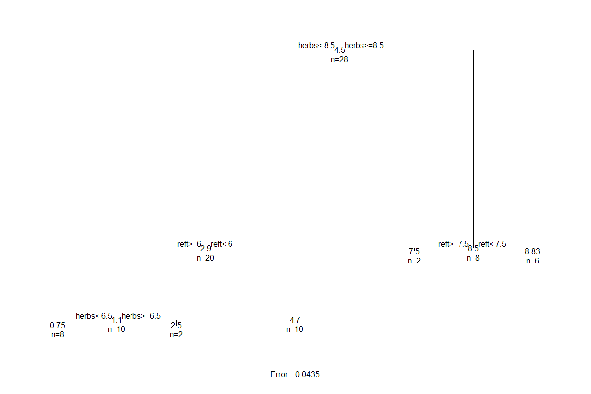
This tree is a helpful visualization of the numerical summary that we saw earlier.
- The lengths of the vertical branches of the tree are proportional to the amount of variation explained by that split (analogous to how the vertical axis in a dendrogram is proportional to the amount of variation explained by a cluster).
- At each intermediate node, the variable selected to split the dataset is shown, along with the value at which it splits it.
- At leaves (terminal nodes), the numbers are the mean value of the response (abundance of T. terricola in this case) and the number of sample units in that group.
Plotting Using ggplot2
Here is an example of how to draw a regression tree using ggplot2 and ggdendro. We already loaded ggplot2 as part of tidyverse; we now need to (possibly install and then) load ggdendro:
library(ggdendro)
The ggdendro package includes a function, dendro_data(), that organizes the components of a dendrogram in an object of class ‘dendro’:
ddata <- dendro_data(Troc.terr)
By inspecting this object, you can see that it contains three key sub-objects:
segments– the coordinates for drawing the tree itself.labels– the data to report at each non-leaf node, and the coordinates of each such node.leaf_labels– the data to report at each leaf (terminal node), and the coordinates of each leaf.
To draw the tree, we will call each sub-object within a separately line of code:
ggplot() +
geom_segment(data = ddata$segments,
aes(x = x, y = y, xend = xend, yend = yend)) +
geom_text(data = ddata$labels,
aes(x = x, y = y, label = label), size = 4, vjust = -0.5) +
geom_text(data = ddata$leaf_labels,
aes(x = x, y = y, label = label), size = 4, vjust = 1) +
theme_dendro()
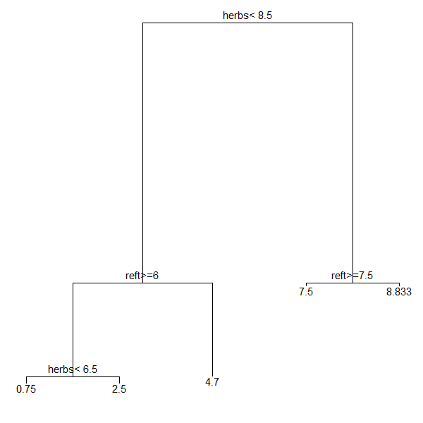
Once you have a base graph like this, you can use the other capabilities of ggplot2 to customize it as desired.
This code can also be easily modified for application to dendrograms from hierarchical cluster analyses.
Plotting Using Base R Capabilities
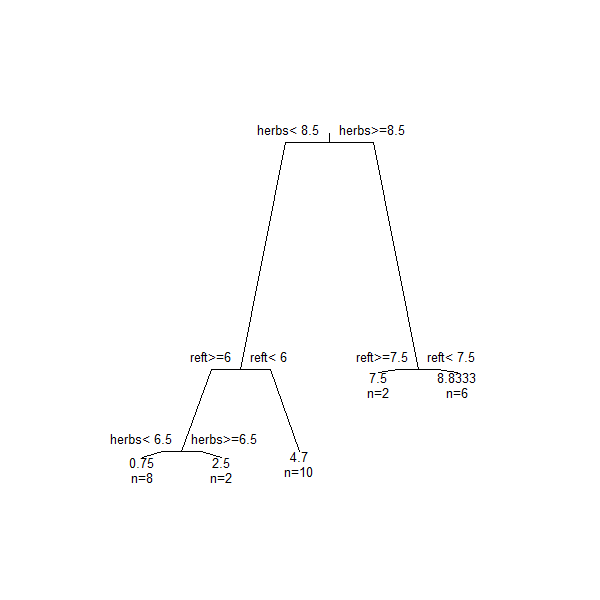
Using the base R plotting functionality to plot the tree, we plot the skeleton of the tree first and then add the textual labels to it. We can also customize many elements of the plot, such as the angle of the branches:
plot(Troc.terr, branch = 0.5, margin = 0.1)
text(Troc.terr, use.n = TRUE, cex = 0.8)
Arguments to customize the skeleton of the tree (i.e., plot()) include:
branch– shape of branches; ranges from 1 (square-shouldered branches) to 0 (V-shaped branches).margin– amount of white space to leave around borders of tree. Helpful if you have long labels.uniform– we didn’t use this here, but setting itTRUEresults in a tree in which the vertical branches are not proportional to the amount of variation explained. Also applies to thetext()function.
Arguments to customize the textual labels (i.e., text()) include:
use.n– whether to include the sample size in each leaf.cex– amount to expand characters. Values < 1 make the text smaller.all.leaves– whether to report the mean value and sample size in every node (TRUE) or just in the leaves (FALSE).
Other options also exist; see ?plot.rpart and ?text.rpart for details.
Cross-Validation
Theory and Considerations
The above tree provided an introduction to the overall structure of these objects. However, it may not be optimally sized. Classification and regression trees are overly ‘optimistic’ in their ability to classify objects, and thus it is preferable to test trees using data that were not part of their construction. This process is called cross-validation. Specifically, cross-validation involves:
- Omitting a subset of the data
- Building a tree from the rest of the dataset
- Examining how well the tree predicts or classifies the omitted subset
Model fit is expressed as relative error, as above. The tree with the smallest cross-validated error should give the most accurate predictions. However:
- Cross-validated relative error cannot be smaller than the relative error for a tree of a given size
- While relative error decreases as the tree gets more complex, this is not necessarily the case for cross-validated relative error.
There are three aspects of cross-validation to consider.
- How many groups to split the data into? The default is
xval = 10, but if the the dataset is small, Borcard et al. (2018) suggest using as many groups as there are samples in the dataset. The help file indicates thatxvalcan be specified as an argument directly withinmvpart()or withinrpart.control(). However, my testing indicates that calling it directly inmvpart()does not alter the results (comparex$control$xvalof modelxwith and without this argument). I therefore recommend calling it inrpart.control()as shown below. - How to assess the consistency of the cross-validation process itself? This can be done by repeating the cross-validation procedure a specified number of times (
xvmult). The default isxvmult = 0. Note that it appears to me that this is only helpful if you have used fewer cross-validations than are possible (i.e., than there are samples in the dataset). You can explore this by altering the settings below. - How to use the results of the cross-validation. We can either allow the function to automatically choose the solution (
xv = "min"orxv = "1se"; see definitions above), or interactively choose it ourselves (xv = "pick"). When doing this interactively, an overly large tree is grown – i.e., the tree is overfit – and the complexity parameter (cp) is calculated for each tree size. See below for an example and explanation of the resulting figure.
If you use fewer cross-validations than are possible from your dataset, the optimal size of tree can vary from run to run. One way to make your results reproducible – generating the same solution each time – is to use set.seed() to set the random number generator immediately before running mvpart().
Key Takeaways
Cross-validation is critical for assessing how well a URT can classify (predict the group identity) of new observations.
Illustration
We’ll specify the number of times the cross-validation process is repeated (xvmult) and the number of cross-validations (xval), and interactively choose the size of the desired tree (xv = "pick"):
Troc.terr.xv <- mvpart(spider[,"troc.terr"] ~ .,
data = env,
xv = "pick",
xvmult = 100,
control = rpart.control(xval = nrow(spider)/2),
all.leaves = TRUE,
plot.add = TRUE)
The xval argument sets the cross-validations to use half of the data. Note that this is specified within the rpart.control() function as a response to the control argument.
The xvmult argument alters the cp graph by adding bars showing how many of the multiple cross-validations identified a tree of that size as having the minimum cross-validated relative error. This information is also reported in the Console.
A graph of the cp table is displayed on the screen:

Some notes about this image:
- The green line is the relative error, as we saw previously
- The blue line is the cross-validated relative error
- The red horizontal line is one SE above the minimum cross-validated relative error
- The red point indicates the tree size that resulted in the smallest cross-validated relative error
- The orange point indicates the smallest possible tree that is below the red line (i.e., within one SE of the minimum cross-validated relative error)
- The green vertical lines descending from the top of the graph are a histogram showing how many of the cross-validations produced a tree in which the smallest cross-validated relative error was for that size. In this case, about equal numbers produced trees of size 3 or 4, and a few produced a tree of size 5.
At this point, R expects you to click on the plot to select the size of tree that you want to produce. Until you do so, the Console will be busy and will not recognize other commands. Once you have selected the size of tree that you want to produce, the rest of the function executes, and the plot of the cp table is replaced with the resulting tree.
Pruning a Tree
Arguments such as minsplit and minbucket provide controls on the size of the leaves that result from a regression tree. They each have defaults as described above – unless over-written, nodes are not split if they contain fewer than 5 observations (minsplit = 5) and every terminal node must have one-third of the observations in the preceding node (minbucket = round(minsplit/3)).
Pruning can be performed manually with the snip.rpart() function. This can be done graphically or by using the toss argument, which refers by number to the node(s) at which snipping is to occur.
snip.rpart(Troc.terr, toss = 2)
n= 28

node), split, n, deviance, yval
      * denotes terminal node

1) root 28 263.0000000 4.500000
  2) herbs< 8.5 20  79.8000000 2.900000 *
  3) herbs>=8.5 8   4.0000000 8.500000
    6) reft>=7.5 2   0.5000000 7.500000 *
    7) reft< 7.5 6   0.8333333 8.833333 *
By comparing this object with and without snipping, you can see that this function does not display further branching from node 2 but shows the branching from node 3. This is applied to the tree that you’ve already created, so the node numbers aren’t changed (i.e., nodes 4 and 5 are absent in the above tree). See the help files for more information.
To snip at multiple nodes, simply include those nodes together:
snip.rpart(Troc.terr, toss = c(3,4))
n= 28

node), split, n, deviance, yval
      * denotes terminal node

1) root 28 263.0 4.5
  2) herbs< 8.5 20  79.8 2.9
    4) reft>=6 10   6.9 1.1 *
    5) reft< 6 10   8.1 4.7 *
  3) herbs>=8.5 8   4.0 8.5 *
Here, we have specified not to split nodes 3 and 4 into smaller nodes, so they are treated as terminal nodes.
Conclusions
Univariate regression trees (URTs) are conceptually different than many other techniques that you’ve probably encountered. They can be used to evaluate a large number of explanatory variables and identify those that most strongly distinguish groups of observations with similar responses. The structure of the tree can depend strongly on which explanatory variables are included in it – particularly if they are the basis for early splits as they will determine which observations are part of each subsequent branch. Explanatory variables that are not included in the tree do not affect it.
URT is a divisive approach – it looks for ways to split a node – and is hierarchical – a split that happens early in the process constrains all subsequent decisions within the resulting nodes.
The theory behind URTs is also directly relevant for multivariate regression trees, which we consider next.
References
Borcard, D., F. Gillet, and P. Legendre. 2018. Numerical ecology with R. 2nd edition. Springer, New York, NY.
De’ath, G. 1999. Extended dissimilarity: a method of robust estimation of ecological distances from high beta diversity data. Plant Ecology 144:191–199.
De’ath, G. 2002. Multivariate regression trees: a new technique for modeling species-environment relationships. Ecology 83:1105-1117.
De’ath, G., and K.E. Fabricius. 2000. Classification and regression trees: a powerful yet simple technique for ecological data analysis. Ecology 81:3178-3192.
Hothorn, T., K. Hornik, and A. Zeileis. 2006. Unbiased recursive partitioning: a conditional inference framework. Journal of Computational and Graphical Statistics 15:651-674.
Vayssières, M.P., R.E. Plant, and B.H. Allen-Diaz. 2000. Classification trees: an alternative non-parametric approach for predicting species distributions. Journal of Vegetation Science 11:679-694.
Media Attributions
- De’ath.2002_Figure3
- URT.root
- URT.root.all.splits
- URT.split2.5
- URT.split5.5
- URT.split7.5
- URT.2split2.5
- mvpart.cp
- URT
- URT.troc.terr
- URT.troc.terr.gg
- URT.troc.terr.baseR
- URT.xv.pick
