
Group Comparisons
17 ANOSIM
Learning Objectives
To understand the theory behind ANOSIM.
To apply ANOSIM manually and through R.
Key Packages
require(vegan)
Theory
ANalysis Of SIMilarity (ANOSIM) was proposed by Clarke & Green (1988). It can be used to determine whether there are statistically significant differences between two or more groups. ANOSIM is a non-parametric technique based on ranks. You may have encountered non-parametric univariate techniques based on ranks before, such as the Kruskal-Wallis test or the Mann-Whitney U test. We will encounter ranked data again in a few weeks when we discuss non-metric multidimensional scaling (NMDS).
The key idea behind ANOSIM is that if the grouping variable is important, then on average the rank distance within groups will be smaller than the rank distance between sample units from different groups.
Recent ecological examples are provided by Muthukrishnan et al. (2019), who compared marine microbial communities, and Sun et al. (2019), who compared soil fungal assemblages beneath different shrubs.
ANOSIM has lower power (higher probability of Type II statistical error) if strong gradients are present in the data (Gotelli & Ellison 2004). See the end of this chapter for recent developments with this technique.
As available in R, ANOSIM is limited in its utility as it can only be used for one-way and fully crossed or nested two-way designs.
Key Takeaways
ANOSIM is a non-parametric test based on the rank distances among sample units. If a grouping variable is important, the mean rank distance among sample units within a group will be smaller than the rank distance between sample units from different groups.
The test statistic (R) ranges from -1 (all lowest ranks are between groups – an unusual situation) to +1 (all lowest ranks are within groups).
A generalized ANOSIM statistic can be applied to complex designs with 2 or 3 factors.
Basic Procedure
The basic procedure for ANOSIM is as follows:
- Begin with a distance matrix. Convert the distances within the matrix to their ranks, such that the smallest distance has a rank of 1.
- Group the ranks to distinguish those that represent observations within the same group and those that represent observations from different groups.
- Calculate the average rank within groups ([latex]\bar r_{W}[/latex]) and the average rank between groups ([latex]\bar r_{B}[/latex]). If the grouping factor is important, the mean rank within groups should be smaller than the mean rank between groups. Can you see why this is so?
- Calculate and save the ANOSIM test statistic, R (confusing; not the software!):
[latex]R = \frac{\bar r_{B} - \bar r_{W}}{n (n - 1) / 4}[/latex]
R ranges from -1 if all of the lowest ranks are between groups to +1 if all of the lowest ranks are within groups. It is zero if the high and low ranks are perfectly mixed between and within groups. - Test the significance of R via permutations:
- Shuffle the order of the values in the grouping factor.
- Recalculate R using the permuted grouping factor (i.e., assuming that each observation came from the group specified in the permuted grouping factor). Save this value.
- Repeat: reshuffle and recalculate the specified number of times. The permutations produce a sampling distribution of R against which the actual test statistic is compared.
- Calculate the P-value as the proportion of permutations that yielded an R equal to or stronger than the R calculated from the actual data.
Simple Example, Worked by Hand
We’ll start with the dissimilarity matrix based on the two response variables:
Resp.dist <- dist(perm.eg[ , c("Resp1", "Resp2")])
| Plot1 | Plot2 | Plot3 | Plot4 | Plot5 | |
| Plot2 | 2.828 | ||||
| Plot3 | 4.123 | 2.236 | |||
| Plot4 | 11.314 | 11.662 | 9.849 | ||
| Plot5 | 9.849 | 9.220 | 7.071 | 4.123 | |
| Plot6 | 12.207 | 12.042 | 10.000 | 2.236 | 3.162 |
For clarity, distances between plots from different groups are shown in bold (compare with the group identities to verify this).
Now, we replace the distances with their ranks. Tied values are given the average of the two ranks. The distances between plots from different groups are again shown in bold.
| Plot1 | Plot | Plot3 | Plot4 | Plot5 | |
| Plot2 | 3 | ||||
| Plot3 | 5.5 | 1.5 | |||
| Plot4 | 12 | 13 | 9.5 | ||
| Plot5 | 9.5 | 8 | 7 | 5.5 | |
| Plot6 | 15 | 14 | 11 | 1.5 | 4 |
We can use this to calculate the average rank within and between groups:
- Within groups: [latex]\bar r_{W} = \frac{3 + 5.5 + 1.5 + 5.5 + 1.5 + 4}{6} = 3.5[/latex]
- Between groups: [latex]\bar r_{B} = \frac{12 + 9.5 + 15 + 13 + 8 + 14 + 9.5 + 7 + 11}{9} = 11[/latex]
Calculate R:
[latex]R = \frac{\bar r_{B} - \bar r_{W}}{n (n - 1) / 4} = \frac{11 - 3.5}{6 ( 6 - 1) / 4} = \frac{7.5}{7.5} = 1[/latex]
Inspection of the ranked distance matrix shows that every small rank is among observations in the same group, which is why R is at its maximum possible value. The statistical significance of this statistic would be assessed with a permutation test.
Implementation in R (vegan::anosim())
In R, ANOSIM can be conducted using the anosim() function in the vegan package. The usage of this function is:
anosim(

x,

grouping,

permutations = 999,

distance = "bray",

strata = NULL,

parallel = getOption("mc.cores")

)
The arguments are:
x– an object of class matrix or data frame in which rows are samples and columns are response variable(s), or a dissimilarity object (class dist) or a symmetric square matrix of dissimilaritiesgrouping– factor for grouping observationspermutations– number of permutations to conduct to assess the significance of R, or a list of permutation instructions obtained using thehow()function. This latter option is necessary with complex designs where permutations need to be restricted – see this chapter for details. Default is to conduct 999 permutations without any restrictions to the permutations.distance– distance measure applied to object if it is not a distance matrix. Thevegdist()function is used here, along with its default distance measure, Bray-Curtis. However, any distance measure available throughvegdist()can be specified.strata– integer vector or factor identifying strata that permutations are to be restricted within.parallel– option for parallel processing
If saved, the resulting object is of class ‘anosim’. Objects of this class have pre-defined methods for applying the plot() and summary() functions.
Simple Example, in R
Applying ANOSIM to the distance matrix:
simple.results.anosim <- anosim(x = Resp.dist, grouping = perm.eg$Group, permutations = 999)
simple.results.anosim
Call:anosim(x = Resp.dist, grouping = perm.eg$Group, permutations = 999)
Dissimilarity: euclidean
ANOSIM statistic R: 1 Significance: 0.1Permutation: freeNumber of permutations: 719Do the two groups differ in overall response?
Note the messages that were displayed on the screen while conducting the analysis:
'nperm' >= set of all permutations: complete enumeration.
Set of permutations < 'minperm'. Generating entire set.
This is because we specified 999 permutations but there are only 720 possible permutations of 6 sample units (n!). The permutations argument calls another function which calculates how many permutations are possible. If more were specified than are possible, the entire set of permutations is calculated and evaluated.
Side notes:
- Other packages may allow more permutations. In these cases, some of the permutations would be duplicates. This is ok – since the P-value is a proportion it is minimally affected by how much and which permutations are duplicated – though computationally inefficient.
- It may seem logical to specify that we want 720 permutations since that’s how many are possible, but we do not control the identity of the permutations themselves. For example, a set of permutations could include some duplicates but not include all possible permutations. Therefore, it is preferable to let the function compare the requested and possible permutations.
Grazing Example, in R
Applying ANOSIM to our grazing example:
grazing.results.anosim <- anosim(x = Oak1.dist, grouping = grazing, permutations = 999)
grazing.results.anosim
Call:
anosim(x = Oak1.dist, grouping = grazing, permutations = 999)
Dissimilarity: bray
ANOSIM statistic R: 0.1333
Significance: 0.015
Permutation: free
Number of permutations: 999
Is there a relationship between current grazing status and community composition?
The P-value is the proportion of permutations that resulted in a value of R as large or larger than that calculated using the actual grouping factor. Note that the P-value differs slightly among individual runs of this test due to differences in which permutations were used.
Rerun this test with differing numbers of permutations (9, 99, 999, 9999). How does the P-value change? Does the correlation itself change?
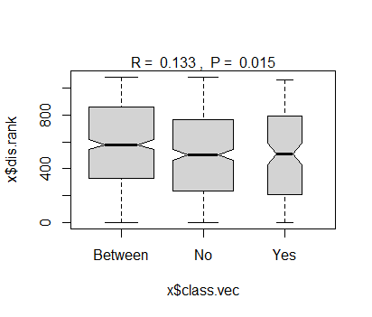
The plot() function generates different products based on the class of the object to which it is applied. When applied to an object of class ‘anosim’:
plot(grazing.results.anosim)
More detailed results from this analysis can be viewed with the summary() function:
summary(grazing.results.anosim)
Call:
anosim(x = Oak1.dist, grouping = grazing, permutations = 999)
Dissimilarity: bray

ANOSIM statistic R: 0.1333
      Significance: 0.015

Permutation: free
Number of permutations: 999

Upper quantiles of permutations (null model):
   90%    95%  97.5%    99%
0.0653 0.0906 0.1159 0.1390

Dissimilarity ranks between and within classes:
        0%    25% 50%    75% 100%   N
Between  2 328.75 580 859.75 1079 510
No       1 238.00 504 766.50 1081 435
Yes      3 211.50 509 793.25 1058 136
The summary() function does not display all of the results from this analysis. More details can be seen by investigating the structure of the results object:
str(grazing.results.anosim)
Items within the results object can be individually indexed and used in other functions. For example:
grazing.results.anosim$statistic # The test statistic R
grazing.results.anosim$perm # Values from permutations
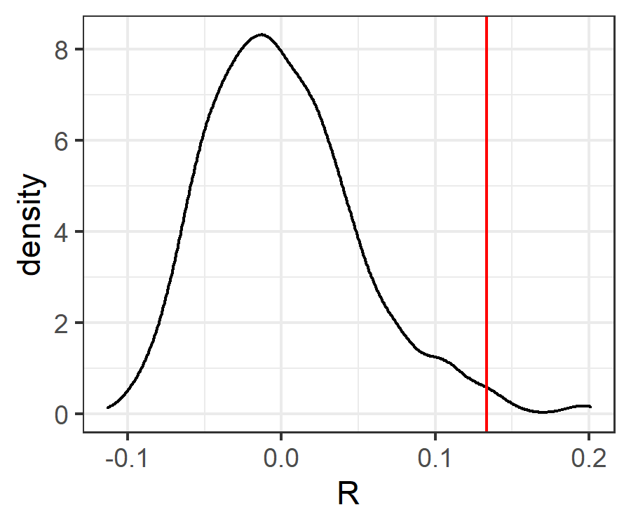
Let’s look at how the test statistic compares with the distribution of values obtained from permutations. To visualize this, we first need to combine the calculated values of the statistic and save them in a data frame.
R.values <- with(grazing.results.anosim, data.frame(R = c(statistic, perm) ) )
R.values$Type <- c("actual", rep("perm", length(R.values$R) - 1))
Now, we can plot these data. We’ll create a density estimate (smoothed histogram) of the values of the test statistic as obtained from the permutations, and superimpose onto it a vertical line showing the value obtained with the real data.
ggplot(data = R.values, aes(x = R)) +
geom_density() + # permuted P-values
  geom_vline(data = R.values[R.values$Type == "actual" , ],

aes(xintercept = R), colour = "red") +
theme_bw()
ggsave("graphics/ANOSIM.R.png", width = 3, height = 2.5, units = "in", dpi = 300)
Recent ANOSIM Developments
A Generalized ANOSIM Statistic
Recent work has proposed a generalized ANOSIM statistic, [latex]R^{\circ}[/latex]. It is defined as “the slope of the linear regression of ranked resemblances from observations against ranked distances among samples, the latter from a simple model matrix assigning the values 1 and 0 to between- and within-group distances, respectively” (Somerfield et al. (2021a, p. 901). If applied to a simple design (e.g., a single factor with two levels, as in our grazing example), it returns the same test statistic as the original R statistic. However, it can also be applied to more complex designs (see below). This test statistic is still permutation-based and, when applied to complex designs, the permutation procedures need to reflect those designs.
The generalized [latex]R^{\circ}[/latex] statistic is still a correlation with a maximum value of 1. It achieves its maximum value if “all dissimilarities between groups are larger than any within groups … and all dissimilarities between groups which are placed further apart in the model matrix are larger than any dissimilarities between groups which the model puts closer together” (Somerfield et al. 2021a, p.906).
Grazing Example
We’ll illustrate the calculation of this generalized [latex]R^{\circ}[/latex] statistic with our grazing example.
To begin, we have to create a distance matrix tracking whether pairs of stands are in the same grazing treatment or not.
graz.dist <- as.numeric( as.factor( grazing ) ) |>

dist()
Verify that you understand why this object contains the values it contains.
Next, we combine the Bray-Curtis distances between sample units (i.e., compositional dissimilarities) and the distances based on grazing treatment.
Oak.eg <- data.frame(
Resp = Oak1.dist,
Group = graz.dist )
Make sure you understand how many rows this object has, and why.
Next, we convert each column of distances into ranks:
Oak.eg <- Oak.eg |>
mutate(Resp.rank = rank(Resp),
Group.rank = rank(Group))
head(Oak.eg)
       Resp Group Resp.rank Group.rank
1 0.3130190     1         2      826.5
2 0.4395344     0         9      286.0
3 0.5988716     1       193      826.5
4 0.8355293     1       965      826.5
5 0.5622599     0       126      286.0
6 0.4604209     0        15      286.0
Each of the new columns is a set of ranks. There are many repeated values due to ties – for example all ranks in Group were either 0 or 1 so there are only two values in Group.rank.
Now, fit a linear model to the ranks:
lm(Resp.rank ~ Group.rank, data = Oak.eg)
Call:
lm(formula = Resp.rank ~ Group.rank, data = Oak.eg)

Coefficients:
(Intercept)   Group.rank
   468.8704       0.1333
The slope of this model is the same value as the ANOSIM test statistic that we calculated earlier (grazing.results.anosim$statistic).
It may also be helpful to graph these ranks against one another, and fit this line to the data.
Extensions of ANOSIM
Somerfield et al. (2021a, b, c) published a series of related articles explaining how this generalized ANOSIM can be applied in a variety of settings.
Ordered factors – an ordinal factor with more than two levels. For example, samples along an environmental gradient (distance from oil rig: > 3.5 km, 1-3.5 km, 0.25-1 km, or < 0.25 km), or times along a time series (sites representing a long-term gradient in heavy metal contamination) (Somerfield et al. (2021a).
Two-factor designs – including nested and crossed designs, with or without ordered factors, and with or without subsampling (Somerfield et al. 2021b). This article notes that ANOSIM is fully non-parametric and cannot test interactions; instead it “provides a robust, comparable and globally interpretable measure of magnitude of overall community change associated with each factor, having excised any possible effect from the factor(s) it is crossed with, irrespective of whether the factors interact or not” (p. 911). Their Table 1 provides details for four 1-factor designs and fourteen 2-factor designs, with examples. It is reprinted in Appendix 2.
Three-factor designs – this is an extension of the 2-way design to include a third factor (Somerfield et al. 2021c). Their Table 1 provides details for thirteen 3-factor designs, with examples. It is reprinted in Appendix 2.
These extensions highlight the utility of the generalized ANOSIM for ordered factors and note that analysis of a genuinely ordered factor will be more powerful if that ordering is incorporated into the test design (but conversely analyses would be less powerful if applied to genuinely unordered factors).
Unfortunately, to my knowledge these extensions are not currently available in R. The examples provided in the articles cited here were conducted in PRIMER, a commercially available software package.
The design considerations highlighted in these tables are also relevant for other techniques.
References
Clarke K.R., and R.H. Green. 1988. Statistical design and analysis for a ’biological effects’ study. Marine Ecology Progress Series 46:213-226.
Gotelli, N.J., and A.M. Ellison. 2004. A primer of ecological statistics. Sinauer, Sunderland, MA.
Muthukrishnan, T., M. Al Khaburi, and R.M.M. Abed. 2019. Fouling microbial communities on plastics compared with wood and steel: are they substrate- or location-specific? Microbial Ecology 78:361-379.
Somerfield, P.J., K.R. Clarke, and R.N. Gorley. 2021a. A generalized analysis of similarities (ANOSIM) statistic for designs with ordered factors. Austral Ecology 46:901-910.
Somerfield, P.J., K.R. Clarke, and R.N. Gorley. 2021b. Analysis of similarities (ANOSIM) for 2-way layouts using a generalized ANOSIM statistic, with comparative notes on Permutational Multivariate Analysis of Variance (PERMANOVA). Austral Ecology 46:911-926.
Somerfield, P.J., K.R. Clarke, and R.N. Gorley. 2021c. Analysis of similarities (ANOSIM) for 3-way designs. Austral Ecology 46:927-941.
Sun, Y., Y. Zhang, W. Feng, S. Qin, and Z. Liu. 2019. Revegetated shrub species recruit different soil fungal assemblages in a desert ecosystem. Plant and Soil 435:81-93.
Media Attributions
- grazing.results.anosim
- ANOSIM.R
