Introduction

PERmutational Multivariate ANalysis of VAriance (PERMANOVA) is a permutation-based technique - it makes no distributional assumptions about multivariate normality or homogeneity of variances.  It can be thought of visually or geometrically.

PERMANOVA is equivalent to MRPP under certain conditions (Reiss et al. 2009), but is much more versatile and widely applicable.  Understanding its versatility requires also considering its flexibility and its limitations.  PERMANOVA can be used to analyze complex models, including multiple factors, covariates, and interactions between terms.  More information about this is provided in the chapters about complex designs and restricting permutations.

Laughlin et al. (2004) provide an example of how these techniques can be applied to plant community data with repeated measurements (i.e., compositional data from permanent plots sampled in multiple years).  Hudson & Henry (2009) used adonis() while Assis et al. (2018) used adonis2(); we discuss both of these functions below.  Sharma et al. (2019) use both PERMANOVA (though they don’t specify which function within vegan) and anosim() to examine the microbiome of people and their built environment.

Theory

Calculating Variation

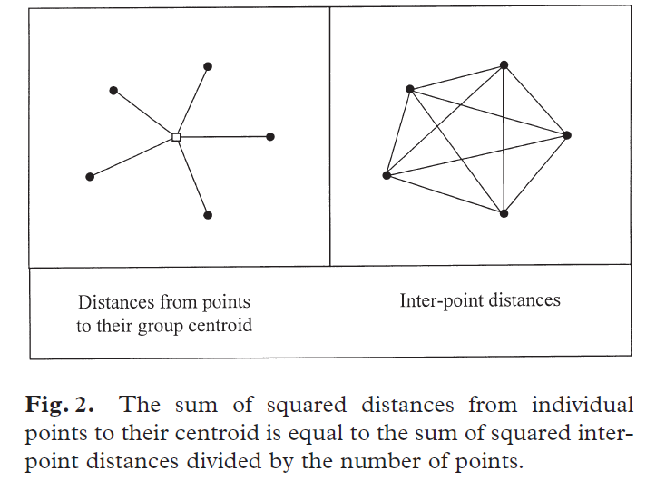
Recall that ANOVA quantifies the variation within a dataset as the sum of squared differences between points and their mean or centroid.  The key insight behind PERMANOVA is that the variation within a group can also be calculated directly from a distance matrix.  Specifically, the sum of squared differences between points and their centroid is equal to the sum of the squared interpoint distances divided by the number of points.  This idea is illustrated below (Fig. 2 from Anderson 2001).  It is known as Huygens’ theorem as it was first formulated by Christiaan Huygens in the 17th century (Anderson et al. 2008)!  Anderson (2015) describes this as geometric partitioning. 

For metric distance measures (e.g., Euclidean distance), these two approaches provide identical answers.

For semimetric distance measures (e.g., Bray-Curtis dissimilarity), the situation is more complicated.  These measures do not satisfy the triangle inequality (please review the Distance Measures chapter if this does not sound familiar), which means that we cannot determine the locations of centroids from the locations of the data.  We therefore cannot calculate the variation within a dataset expressed by one of these measures using the conventional ANOVA approach.  However, we can use the distance matrix to calculate the variation within the dataset.

Geometric partitioning avoids the need to calculate centroids while yielding the same measure of variation.  By avoiding this step, basic ANOVA theory can be applied to data summarized with any distance measure.  More details, including additional information about the mathematics of PERMANOVA, can be found in Anderson (2001, 2017), McArdle & Anderson (2001), and Anderson et al. (2008).

Partitioning Variation

In ANOVA, the total variation in a dataset (total sum of squares; SST) is based on the differences between points and the grand mean.  This variation is partitioned into the variation within groups (SSW) and the variation between/among groups (SSB).  SSW is calculated based on the differences between points and their group means.  SSB is calculated by subtraction, since these terms are additive:

SST = SSB + SSW

PERMANOVA uses geometric partitioning of the distance matrix to partition variation among sources.  We can calculate SST, SSB, and SSW as with ANOVA.  However, the  resulting technique requires no assumptions about normality and/or homogeneity of variances.  The only assumption is that observations are interchangeable under the null hypothesis – the same assumption as with all permutation tests, and the justification for using permutations to assess significance.

The PERMANOVA test statistic, pseudo-F, is modeled directly after the conventional ANOVA F-statistic.  It is calculated in the same way, as a ratio of the amount of variation between versus within groups, with the numerator and denominator each weighted by their degrees of freedom.  It is 0 or positive, with larger values corresponding to larger proportional importance of the grouping factor.  As with other permutational techniques, the distribution of the test statistic is assessed by repeatedly relabelling observational units (i.e., permuting group identities) and recalculating the test statistic. 

Since it is based on the distance matrix, PERMANOVA can be applied identically to both univariate and multivariate data.  This provides versatility but it also provides reassurance: the test statistic is identical to the conventional F-statistic when calculated using Euclidean distance for a single variable.

Basic Procedure

The basic procedure for PERMANOVA is as follows.

1. Convert data matrix to a distance matrix, using an appropriate distance measure.
2. Square the distance matrix.
3. Calculate three partitions of the variation:
   • Total variation (total sum of squares; SST) - the sum of squared distances divided by the number of plots.
   • Variation within groups (sum of squares within groups; SSW) - calculated identical to SST but separately for each group. Add the value from each group together to yield the overall SSW.
   • Variation between groups (sum of squares between groups; SSB) - calculated by simple subtraction (i.e., SSB = SST – SSW).

4. Calculate the test statistic. The test statistic is termed a ‘pseudo-F statistic’ to distinguish it from the traditional parametric univariate F-statistic, but is calculated using the same formula:
   [latex]PseudoF = \frac{SSB / (t - 1)}{SSW / (N - t)}[/latex]
   where SSB and SSW are as calculated above, t is the number of groups, and N is the total number of sample units.

5. Assess statistical significance via a permutation test:
   • Permute group identities.
   • Recalculate pseudo-F statistic
   • Repeat the specified number of times. The permutations produce a distribution of pseudo-F values against which the actual pseudo-F statistic value is compared.
6. Calculate the P-value as the proportion of permutations that yielded a pseudo-F value equal or greater than the actual data did.

Simple Example, Worked By Hand

Using the data and group identities from our simple example, let’s work through the calculations involved with PERMANOVA.

We begin with our distance matrix.  For clarity, the distances between plots from different groups are in bold (view perm.eg$Group to confirm this).
d.eg <- dist(perm.eg[ , c("Resp1", "Resp2")])

Square the distance matrix to yield squared distances among plots.
d.eg_2 <- d.eg^2

Sum the squared distances and divide by the number of plots to obtain the total sum of squares (SST):

[latex]SST = \frac{1049}{6} = 174.83[/latex]

SST <- sum(d.eg_2) / length(perm.eg$Group)

Note that this is Huygens’ theorem in action!

We obviously could combine these steps.  For example, here's a function to combine all of these steps:

SS.calculation <- function(x, variables) {
require(tidyverse)
n <- nrow(x)
x |>
  dplyr::select(all_of(variables)) |>
  dist() |>
  crossprod() / n

SS.calculation(x = perm.eg,
variables = c("Resp1", "Resp2"))

[1] 174.8333

Review the order of operations as outlined in the function.  This function is available in the GitHub repository.

Now let's calculate the variation within each group (i.e., SSW).  We can manually identify the appropriate squared distances from the above matrix and do the calculation:

[latex]SSW = \frac{8 + 17 + 5}{3} + \frac{17 + 5 + 10}{3} = \frac{30}{3} + \frac{32}{3} = 20.67[/latex]

Or, we can use SS.calculation() to calculate the variation within each group - all we need to do is index the object to refer to the group of interest:

SSW.A <- SS.calculation(x = perm.eg |> filter(Group == "A"),
variables = c("Resp1", "Resp2"))

SSW.B <- SS.calculation(x = perm.eg |> filter(Group == "B"),
variables = c("Resp1", "Resp2"))

SSW <- SSW.A + SSW.B

Calculate the variation between groups (SSB) as the difference between SST and SSW:

[latex]SSB = SST - SSW = 174.83 - 20.67 = 154.16[/latex]

SSB <- SST - SSW

Finally, calculate the pseudo-F statistic:

[latex]PseudoF = \frac{SSB / (t - 1)}{SSW / (N - t)} = \frac{154.16 / 1}{20.67 / 4} = 29.83[/latex]

pseudo.F <- (SSB / (2 - 1)) / (SSW / (6 - 2))

Often, we will summarize this information in an ANOVA table:

This table contains all of the data that we usually see in an ANOVA output except the P-value.  Statistical significance will be determined by permuting the group identities, recalculating the pseudo-F statistic for each permutation, and comparing the observed value against the distribution of values obtained via permutation.

Can you figure out what the pseudo-F statistic is for the permutation of group identities {A,B,A,A,B,B}?  As a hint, the squared distance matrix is repeated here, with bold text to indicate distances between plots from different groups.

Implementation in R

PERMANOVA is becoming increasingly common in community ecology.  It is surprising, therefore, that only a few R packages provide it.  We are using the primary one, vegan.

The LDM (linear decomposition model) package provides another formulation of PERMANOVA. The authors claim that their formulation outperforms those in vegan.  It was developed for use with microbiome data and seeks to simultaneously test global hypotheses (i.e., overall assessment of compositional differences among treatments) and individual operational taxonomic units (OTUs; i.e., response variables) (Hu & Satten 2020).  It has not been updated since 2023, so I am not that it is being maintained.  I have not evaluated this package.

The PERMANOVA package was released in 2021 (Vicente-Gonzalez & Vicente-Villardon 2022) but has not been updated since then.  I have not evaluated this package.

Several other packages also offer permutational multivariate analysis of variance and appear to be independent, but require the vegan package so often (I’ve not verified all) are using vegan’s functions.  These include:

• GUniFrac – this package provides Generalized UniFrac distances for comparing microbial communities (Chen et al. 2012). The package description states that it provides three extensions to PERMANOVA:
  • adonis3() - PERMANOVA with a different permutation scheme (Freedman-Lane)
  • PermanovaG() - an omnibus test using multiple matrices
  • PermanovaG2() - an analytical approach for approximating the PERMANOVA p-value
• RVAideMemoire – this package provides miscellaneous functions useful in biostatistics.  According to the help files:
  • adonis.II() is a wrapper to vegan::adonis2() but performs type II tests (whereas vegan::adonis2() performs type I and type III tests).
  • perm.anova() sounds like a promising function, but appears to be a permutation-based ANOVA.  In other words, it is for a univariate rather than a multivariate response.
• biodiversityR – this package provides a graphical user interface (GUI) for community analysis – this can be useful in the moment but is difficult to script. Its website includes a downloadable book (Kindt & Coe 2005) about the analysis of community data, focusing specifically on trees.  The PERMANOVA functions here are nested.npmanova() and nested.anova.dbrda().
• smartsnp - this package is for genomic data.  The function smart_permanova() is based on vegan::adonis2().

vegan::adonis2()

Early versions of vegan used a function called adonis().  This function is no longer available as of version 2.7-0.  As indicated by its name, adonis2() is a replacement for this older function.  Its usage is:

adonis2(
formula,
data,
permutations = 999,
method = "bray",
sqrt.dist = FALSE,
add = FALSE,
by = NULL,
parallel = getOption("mc.cores"),
na.action = na.fail,
strata = NULL,
...
)

The main arguments are:

• formula – model formula such as Y ~ A + B * C.  See the 'Complex Models' chapter for more details of how to specify a model formula.  For now, the key point is that we are specifying that we want to analyze the response (Y) as a function of (~) one or more explanatory variables (A, B, C).  The class of Y determines what is done:
  • If Y is a dissimilarity matrix (i.e., output from dist() or vegdist()), the pseudo-F statistic is calculated directly.
  • If Y is a data frame or matrix containing data, vegdist() is applied to calculate the distance matrix first and then the pseudo-F statistic is calculated.

• data – the data frame in which the explanatory variables are located.  Sample units are assumed to be in the same order in data as in the rows of Y.
• permutations – number of permutations to conduct to assess the significance of the pseudo-F statistic, or a list of permutation instructions obtained using the how() function.  This latter option is particularly important for PERMANOVA, as it is necessary when permutations need to be restricted - see that chapter for details.  Default is to conduct 999 permutations without any restrictions to the permutations.
• method – method of calculating the distance matrix, if needed (i.e., if Y in the formula is not a distance matrix).  The vegdist() function is used to do these calculations, which is why the default is Bray-Curtis, though you can specify any distance method available in vegdist().
• sqrt.dist – take square root of dissimilarities.  This is one way to make semimetric dissimilarities behave in a more ‘Euclidean’ manner.  Default is to not ‘euclidify’ them in this fashion (FALSE).
• add – add a constant to the dissimilarities so that no eigenvalues are negative.  There are two options here, which we’ll discuss in the context of Principal Coordinates Analysis (PCoA).  Default is to not add this value (FALSE).
• by – How to deal with other terms when assessing significance.  See below for additional discussion of types of sums of squares.  Four options are available:
  • NULL – tests all terms together rather than individually.  This is the default as of version 2.7-0; earlier versions had by = "terms" as the default.
  • terms – tests terms in sequential order, from first to last in formula.  This is the Type I or ‘sequential’ sums of squares that you may recall from basic statistics courses.
  • margin – tests the marginal effect of each term, or its effect after accounting for all other terms in the model.  This is Type III or ‘partial’ sums of squares that you may recall from basic statistics courses.  If applied to a model with an interaction term, this returns the interaction term and ignores the main effects.
  • onedf - tests terms as a series of contrasts, each with one df.
• parallel – option for parallel processing
• na.action - what to do if explanatory variables are missing.  Default is to not continue (na.fail).
• strata – groups that permutations are to be restricted within.  Can alternatively be specified through the permutations() function, which is discussed in this chapter about restricted permutations.

The results from adonis2() are saved to an object of class "anova.cca".  This object is also recognized as belonging to classes "anova" and "data.frame".  It currently includes the degrees of freedom (Df), sums of squares (SumOfSqs), partial R² (R2), pseudo-F statistic (F), and P-value for each term (Pr(>F)) along with the pseudo-F statistics from the permutations (attr(x, "F.perm")) and lots of details about how permutations were conducted.

The partial R² for each term is calculated as the SS for the term as a proportion of SST.  The partial R² values may NOT sum to 1 if you are testing multiple factors using a marginal model (by = "margin") -  see the discussion of types of sums of squares in the 'Complex Models' chapter.

Simple Example

simple.result.adonis2 <- adonis2(
perm.eg[ , c("Resp1", "Resp2")] ~ Group,
data = perm.eg,
method = "euc"
)

Calling this object prints the ANOVA table in the console.

Verify the calculations we made by hand above.  The ANOVA table is identical to what we calculated, though the order of the information is slightly different.  Also, this table includes two elements that we did not calculate:

• The partial R² value for each term. As noted above, this is calculated as the SS for that term as a proportion of the total SS for the dataset.  For example, the partial R² for Group = 154.167 / 174.833 = 0.88179
• A permutation-based P-value for each term being tested (i.e., other than Residual and Total).  Although Group has a large pseudo-F value, it is not statistically significant.  This is a reflection of the limited number of permutations possible given our sample size.

Grazing Example

grazing.result.adonis2 <- adonis2(
Oak1 ~ grazing,
method = "bray"
)

Grazing clearly affects community composition, though it accounts for a relatively small amount of the variation in composition (5.6%).

We did not specify the data argument because grazing was saved as a separate object.  If we wanted to, we could have called it by its column name within Oak (or Oak_explan). Also, if we had specified the distance matrix instead of the data matrix for Y, the method argument would have been unnecessary:

adonis2(Oak1.dist ~ grazing)

Extensions of PERMANOVA

I've introduced PERMANOVA as a means of comparing groups, but it is more broadly described as a linear model.  Recall that ANOVA is a specific instance of a linear model in which the explanatory variable is categorical.  Linear models can be used to compare groups (categorical variables) and to regress one continuously distributed variable on another.  As such, PERMANOVA can be used to analyze any linear model.  This is sometimes referred to more generally as a ‘distance-based linear model’ (DISTLM) or as distance-based redundancy analysis (dbRDA) (Legendre & Anderson 1999; McArdle & Anderson 2001).

The adonis2() function can handle both ANOVA and regression models.  Each variable is treated as categorical or continuous based on its class.  Therefore, it is helpful to always check that the degrees of freedom in a model output correspond to what you expected.  A variable that is categorical will have 1 fewer df than it has levels, whereas a variable that is continuous will only have 1 df.  More information is available in the 'Complex Models' chapter.

Limitations of vegan::adonis2()

Although PERMANOVA is an extremely powerful technique, its implementation in R has some limitations.  Topics like the choice of sums of squares mentioned above are not unique to adonis2().  Two other issues to be aware of are how to handle random effects and how to decide what to permute.  See the chapters about complex models and restricting permutations for help with these issues.

Random Effects

Currently, adonis2() does not permit the specification of random effects.  An alternative way to account for random effects is to use sequential sums of squares and fit the term that would otherwise be designated as a random effect as the very first term in the model.  Doing so results in a model in which as much variation as possible is explained with that term before the other factor(s) are evaluated.  However, using this approach can be ‘expensive’ in terms of df.

For example, if plots were arranged in blocks (e.g., the whole plots of a split-plot design), block ID could be included as the first term in the model so that the variation among blocks is accounted for before testing other terms.  Permutations would also have to be restricted to reflect this design.

Choice of What to Permute

In our earlier examples of permutations, we permuted the group assignment of each sample unit.  We could alternatively have kept the group assignments unchanged but permuted the rows of the response matrix.  Furthermore, the raw data can be permuted or the residuals obtained from a model can be permuted.  In adonis2(), we are not able to specify which of these methods to use.  However, this is likely a relatively minor issue: Anderson et al. (2008) note that these methods give very similar results.

Non-R Formulations of PERMANOVA

If the limitations of adonis2() are problematic for your analysis, you may want to explore a non-R formulation of PERMANOVA.

The PERMANOVA+ extension to PRIMER is an extremely powerful and versatile way to use PERMANOVA.  It was coded by Dr. Anderson (author of the 2001 article that developed this technique and introduced it to ecological audiences) and includes an extensive help manual (Anderson et al. 2008).  Among other features, it permits you to choose which type of SS you would like to use and to analyze unbalanced data, random effects, etc.  The basic approach requires that you create a design file containing the necessary information for partitioning the data based on the factors and experimental design, and then run the PERMANOVA on the distance matrix, choosing that design file during the analysis.

In PC-ORD, PERMANOVA can be used to analyze fairly simple designs.  Responses are coded in one matrix; factors and other explanatory variables are identified in a second matrix.  Any of the distance measures available through PC-ORD can be used.  Pairwise comparisons can be made to evaluate which groups differ in factors with more than two levels.  I haven't used the current version (version 7), but the formulation of PERMANOVA in version 6 had a number of limitations:

• Requires balanced data (same number of sample units in each group)
• Limited to one or two factors

Tang et al. (2016) presented an extension of PERMANOVA for microbiome data that i) can account for ‘confounders’ (confounding variables that are correlated with both the response matrix and explanatory variables), and ii) can compare conclusions across multiple distance measures simultaneously.  For example, an analysis could compare the conclusions if based on Bray-Curtis distances (weighted by abundance) or on Jaccard distance (based on presence/absence data).  A free program, miProfile, is available through Tang’s website.  It is written in the C language.

Conclusions

PERMANOVA is an extremely powerful and versatile technique.  It has strong parallels with ANOVA and thus its application and interpretation are familiar to most ecologists.

The flexibility of PERMANOVA allows it to be used in complex models, but these models can be used incorrectly - as is also the case with ANOVA and other techniques.  See additional ideas in the chapters about complex models, controlling permutations, and restricting permutations.  The appendix describing the structure of complex experimental designs is also helpful in this regard.

References

Anderson, M.J. 2001. A new method for non-parametric multivariate analysis of variance. Austral Ecology 26:32-46.

Anderson, M.J. 2015. Workshop on Multivariate Analysis of Complex Experimental Designs Using the PERMANOVA+ Add-on to PRIMER v7. PRIMER-E Ltd, Plymouth Marine Laboratory, Plymouth, UK.

Anderson, M.J. 2017. Permutational Multivariate Analysis of Variance (PERMANOVA). Wiley StatsRef: Statistics Reference Online.

Anderson, M.J., and C.J.F. ter Braak. 2003. Permutation tests for multi-factorial analysis of variance. Journal of Statistical Computation and Simulation 73:85-113.

Anderson, M.J., R.N. Gorley, and K.R. Clarke. 2008. PERMANOVA+ for PRIMER: Guide to Software and Statistical Methods. PRIMER-E Ltd, Plymouth Marine Laboratory, Plymouth, UK. 214 p.

Assis, D.S., I.A. Dos Santos, F.N. Ramos, K.E. Barrios-Rojas, J.D. Majer, and E.F. Vilela. 2018. Agricultural matrices affect ground ant assemblage composition inside forest fragments. PLoS One 13(5):e0197697.

Chen, J., K. Bittinger, E.S. Charlson, C. Hoffmann, J. Lewis, G.D. Wu, R.G. Collman, F.D. Bushman, and H. Li. 2012. Associating microbiome composition with environmental covariates using generalized UniFrac distances. Bioinformatics 28:2106-2113.

Hu, Y-J., and G.A. Satten. 2020. Testing hypotheses about the microbiome using the linear decomposition model (LDM). Bioinformatics 36:4106-4115.

Hudson, J.M.G., and G.H.R. Henry. 2009. Increased plant biomass in a high Arctic heath community from 1981 to 2008. Ecology 90:2657-2663.

Kindt, R., and R. Coe. 2005. Tree Diversity Analysis: A Manual and Software for Common Statistical Methods for Ecological and Biodiversity Studies. World Agroforestry Centre (ICRAF), Nairobi, Kenya.

Laughlin, D.C., J.D. Bakker, M.T. Stoddard, M.L. Daniels, J.D. Springer, C.N. Gildar, A.M. Green, and W.W. Covington. 2004. Toward reference conditions: wildfire effects on flora in an old-growth ponderosa pine forest. Forest Ecology and Management 199:137-152.

Manly, B.F.J., and J.A. Navarro Alberto. 2017. Multivariate Statistical Methods: A Primer. Fourth edition. CRC Press, Boca Raton, FL.

McArdle, B.H., and M.J. Anderson. 2001. Fitting multivariate models to community data: a comment on distance-based redundancy analysis. Ecology 82:290-297.

Sharma, A., M. Richardson, L. Cralle, C.E. Stamper, J.P. Maestre, K.A. Stearns-Yoder, T.T. Postolache, K.L. Bates, K.A. Kinney, L.A. Brenner, C.A. Lowry, J.A. Gilbert, and A.J. Hoisington. 2019. Longitudinal homogenization of the microbiome between both occupants and the built environment in a cohort of United States Air Force cadets. Microbiome 7:70.

Tang, Z-Z., G. Chen, and A.V. Alekseyenko. 2016. PERMANOVA-S: association test for microbial community composition that accommodates confounders and multiple distances. Bioinformatics 32:2618-2625.

Vicente-Gonzalez, L., and J.L. Vicente-Villardon. 2022. PERMANOVA: Multivariate Analysis of Variance Based on Distances and Permutations. R Package, v.0.2.0.