
Foundational Concepts
11 Properties of Distance Measures
Learning Objectives
To consider the desirable properties of distance or dissimilarity measures, including the difference between the two.
To introduce the distance matrix as a method of summarizing a set of pairwise distances.
To understand how distance measures use matrix algebra to provide a link between raw data, data adjustments, and techniques to test for statistical differences, identify groups, and visualize patterns.
Introduction
Distance measures are an essential component of many ecological analyses. Here, we’ll review the properties of the distance measures that are most commonly used in ecological studies.
Distance measures can be calculated among plots (aka sample units; the rows in your data matrix) or species (aka variables; the columns in your data matrix). However, most analyses are based on the distances among plots, so that’s what I’ll assume throughout these notes.
Terminology
Many people use the terms ‘distance’ and ‘dissimilarity’ interchangeably, though some authors recommend using ‘distance’ only for metric indices (those that satisfy the triangle inequality – see below).
Similarity is the opposite of dissimilarity. Similarity can only be calculated for metrics which have an upper limit.
Simple Examples
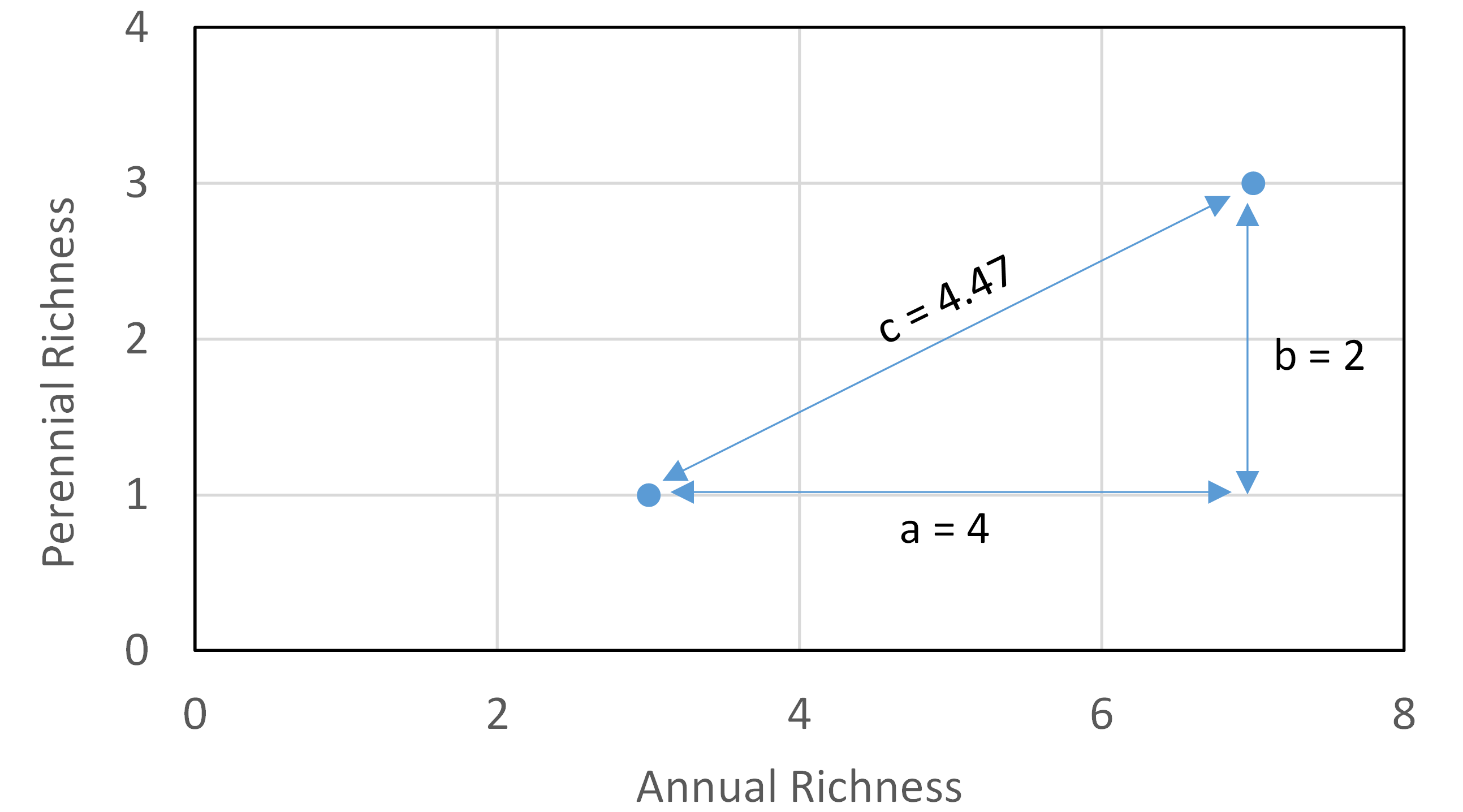
A helpful way to begin thinking about the idea of distance is to consider univariate or one-dimensional data. For example, here are data from two plots:
| Plot | Total Richness |
| H | 4 |
| I | 10 |
These two plots obviously differ by 6 species. This is the distance between the two plots.
Now, suppose that we distinguished annual and perennial plants within each plot:
| Plot | Annual Richness | Perennial Richness |
| H | 3 | 1 |
| I | 7 | 3 |
Total richness is the same as before, but what is the distance between the two plots now?
A reasonable first step is to use the Pythagorean theorem (a2 + b2 = c2) to calculate the Euclidean distance (ED) between the two plots:
[latex]ED = \sqrt{(x_{HA} - x_{IA})^2 + (x_{HP} - x_{IP})^2} = \sqrt{(3 - 7)^2 + (1 - 3)^2} = 4.47[/latex] species
Incorporating information about the longevity of the plant species has reduced the distance between the plots from 6 species to 4.5 species. A visualization of this calculation is shown below.
Desirable Properties of Distance Measures
We will consider five desirable properties of distance measures (more have been suggested – see Legendre & De Cáceres (2013) for details).
1) Zero If Identical
If sample units A and B have the same values for all variables, the distance between them should be zero.
This is true of all distance measures we will consider.
2) Positive
If sample units A and B do not have the same values for all variables (i.e., are not identical), the distance between them should be positive. Since the distance is zero when they are identical (property 1), what would a negative distance mean?
This is true of all distance measures we will consider.
3) Symmetric
A distance measure is symmetric if the distance from A to B equals the distance from B to A.
This is true of all distance measures we will consider. When would a distance measure not be symmetric? Some examples are found in mapping applications. In essence, these applications seek the shortest distance between two points. However, there are multiple scenarios in which the shortest distance between two points is not the same:
- Driving directions, especially when there are one-way streets. The roads you use to get to a location are not the same ones you would use to drive back from that location. This is a special form of the Manhattan or city block distance. More information: https://en.wikipedia.org/wiki/Taxicab_geometry.
- Estimates of travel time between destinations that incorporate elevation and account for the fact that it is more work to walk uphill than downhill. For example, Google maps estimates that it would take 4 minutes less time for me to walk to UW than home from it, probably due both to slightly different route recommendations and to the elevation difference. This example is modified from https://en.wikipedia.org/wiki/Metric_(mathematics)#Quasimetrics.
- As an ecological example, Acevedo et al. (2015) studied a wind-dispersed orchid and showed that models which accounted for wind direction more accurately predicted its colonization and extinction dynamics. In other words, if sample unit A is downwind of sample unit B, the effective distance between them was smaller from B to A than from A to B – pollen would have to travel ‘farther’ upwind from A to B.
Another example of an asymmetric distance is a situation in which we’re interested in the change in a univariate response. For example, imagine that the number of trees is measured multiple times on a plot. We generally would care more about the change in density from an earlier time to a later time. The change from a later time to an earlier time can be calculated mathematically but is of limited utility. This is also a situation in which we would want to use a distance measure that retains the directionality of the change – whether it increased or decreased.
4) Metric or Semimetric?
When we have multiple sample units, we can calculate distances between many pairs of sample units. For example, if we have three sample units (A, B, C), we can calculate the distance from A to B, A to C, and B to C. Imagine the distances between A, B, and C as the sides of a triangle with the vertices representing the sample units.
A metric distance measure follows the principles of Euclidean geometry in what is known as the triangle inequality theorem (see image below): the distance from one sample unit to another (e.g., A to C) is always smaller than the combined distance from the first to the other by way of a third (e.g., A to B and B to C). Measures that satisfy this inequality are most properly referred to as ‘distance measures’.
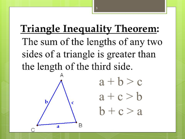
Measures that do not satisfy the triangle inequality theorem are semimetric. With these measures, Euclidean geometry may not work – the distance from A to C can be greater than the combined distance from A to B and B to C. These are properly referred to as ‘dissimilarity measures’. See the Sorenson dissimilarity in the next chapter for an example.
5) Is There a Constant Maximum?
Some measures do not have an upper limit – no matter what the distance is between two sample units, you can conceive of a situation in which the distance would be greater. For example, consider the physical distance between sample units. No matter how far apart two sample units are, you can envision another pair of sample units that are further apart.
Other measures have a constant maximum, meaning that there is no situation in which the distance could be greater. This can happen when samples have no elements in common, and often arises when the distance is expressed as a proportion of some total – doing so bounds the values to be less than or equal to 1. Many of these are dissimilarity measures.
The presence of a constant maximum permits a dissimilarity measure to also be expressed as a similarity measure. For example, if two sample units have a dissimilarity of 0.25 in a measure with a maximum dissimilarity of 1, it would be equivalent to say that they have a similarity of 0.75 (i.e., 1 – 0.25).
The Distance Matrix
When a distance measure is applied to multiple plots, a distance is calculated for every pairwise combination of plots. These distances are then assembled into a distance matrix (or dissimilarity matrix). For example, here is a distance matrix between three plots (A, B, C):
| A | B | C | |
| A | 0.0 | 0.8 | 0.4 |
| B | 0.8 | 0.0 | 0.5 |
| C | 0.4 | 0.5 | 0.0 |
This matrix has several important features:
- It is square – recall from the matrix algebra chapter that many of the manipulations possible with matrix algebra are applied to square matrices.
- It is symmetric (desirable property #3) – for example, the distance from A to B is the same as the distance from B to A. This means that the upper-triangle is a mirror image of the lower-triangle.
- The distance between a plot and itself is zero (desirable property #1) – all values along the diagonal are zero.
- The first row and last column are non-informative – they contain information that is also reported elsewhere in the matrix.
As a result of these features, we often display a distance matrix more concisely as a lower triangular matrix:
| A | B | |
| B | 0.8 | |
| C | 0.4 | 0.5 |
Although this doesn’t look like a matrix and is neither square or symmetric, it is still described as a distance matrix. Furthermore, even though it may appear to have only two rows and two columns it is still a 3 x 3 distance matrix.
A distance matrix summarizes the distances between every pair of sample units.
How does the number of pairwise distances scale with the number of sample units? There are [latex]n \times n = n^2[/latex] pairwise combinations of [latex]n[/latex] sample units. However, since a distance matrix is symmetric with zeroes on the diagonal, the number of unique pairwise combinations is
[latex]\frac{n (n - 1)}{2}[/latex].
How many unique pairwise combinations are there for:
3 sample units? __________
10 sample units? __________
20 sample units? __________
The Distance Matrix
The distance matrix is square and symmetric, with zeroes on the diagonal. Therefore, it is often shown simply as its lower triangle.
The number of pairwise distances in the matrix is a function of the number of sample units.
The number of variables has no effect on the size of the distance matrix.
Conclusions
The calculation of a distance between two sample units compresses or combines all of the differences between two samples into a single number. This ‘compression’ occurs regardless of whether the samples are being compared with respect to a single variable (e.g., species richness) or a multivariate measure (e.g., community composition). Can you see how this is so?
Another way of stating this is that the size of the distance matrix is a function of the number of sample units, not the number of variables. Because a distance matrix is unaffected by the number of variables, distance-based techniques can be applied identically to both univariate and multivariate data; separate techniques are not required as is the case with conventional parametric techniques (e.g., ANOVA vs. MANOVA).
There are many ways to combine the differences between sample units. The next chapter reviews a number of these distance measures.
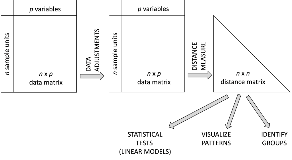
The rest of this course builds upon the foundation laid up to this point. Once we have made all desired data adjustments and expressed the differences among samples in a distance matrix, we can use that distance matrix to test for differences among pre-existing groups, visualize patterns, identify natural groups in the data, etc.
This road map might clarify the process:
References
Acevedo, M.A., R.J. Fletcher Jr., R.L. Tremblay, and E.J. Meléndez-Ackerman. 2015. Spatial asymmetries in connectivity influence colonization-extinction dynamics. Oecologia 179(2):415-424.
Legendre, P., and M. De Cáceres. 2013. Beta diversity as the variance of community data: dissimilarity coefficients and partitioning. Ecology Letters 16:951-963.
Media Attributions
- richness
- triangle.inequality
- analysis.road.map
