Introduction

Univariate and bivariate outliers are relatively easy to detect (e.g., Zuur et al. 2010), but multivariate outliers are much more difficult.  For example, if a dataset contains more than 3 variables, multivariate outliers cannot be detected graphically without first applying some method to reduce the dimensionality of the data.  Creating a distance matrix is one way of doing so.  If a single sample unit is a multivariate outlier, then there will be a large distance between it and all other elements. 

The choice of distance measure will affect the ability to detect outliers.  As an extreme example, an outlier in abundance would not be detectable if the data were summarized using a measure based on presence/absence.

Multivariate outliers can be explored visually and numerically.  We’ll use a hypothetical but realistic example to illustrate an outlier.  We begin by opening our R Project and loading our Oak data:

Oak <- read.csv("data/Oak_data_47x216.csv", header = TRUE, row.names = 1)
Oak_species <- read.csv("data/Oak_species_189x5.csv", header = TRUE)

We’ll focus on the geographic coordinates of the stands.  Let’s calculate the Euclidean distance among the stands:

require(tidyverse); require(vegan)
Oak$Stand <- row.names(Oak)
original.dis <- Oak |>
  dplyr::select(LatAppx, LongAppx) |>
vegdist(method = "euclidean")

What if the decimal place is off by one position in one of the latitude values?  To create this example dataset, we’ll change the first latitude value and then calculate a new distance matrix.  Note that this is a temporary (scripted) adjustment – since we aren’t saving the changed value within Oak, our real data aren’t affected.
outlier.dis <- Oak |>
  mutate(LatAppx = case_when(Stand == "Stand01" ~ LatAppx / 10,
    TRUE ~ LatAppx)) |>
  dplyr::select(LatAppx, LongAppx) |>
vegdist(method = "euclidean")

Heat Maps (coldiss())

Since a distance matrix contains so many values and is difficult to view, several ways have been developed to summarize it graphically.  Borcard et al. (2018) provide a function, coldiss.R, to generate heat maps of a distance matrix.  The function is available in the collection of data, functions, and scripts that they have published on their website.  I have copied it to the course GitHub repository for ease of access.

To use this function:

• Create a ‘functions’ subfolder in your project folder.
• Download and save coldiss.R to this subfolder.
• Open your R project.
• Load this function using the source() function:  source("functions/coldiss.R")

Note that this function is now listed in the Environment panel.  There are four arguments:

• D – distance matrix to use.
• nc – number of colors to use in heat map. Default is to use 4 colors (nc = 4).
• byrank – whether to use equal-sized classes (byrank = TRUE) or to have equal spacing among classes (byrank = FALSE).  For example, imagine that there are 100 distances that those distances range from 0 to 1.  Setting byrank = TRUE means that 250 distances will be in each class; this is the default.  Setting byrank = FALSE means that distances from 0-0.25 will be in one class, 0.25-0.5 in another class, etc.
• diag – whether to print object labels on the diagonal (diag = TRUE). Default is to not do this.

We will apply this function to our outlier.dis distance matrix created above.  Since we are concerned here about the actual values of the distances, we will specify equal spacing among classes:
coldiss(outlier.dis, byrank = FALSE)

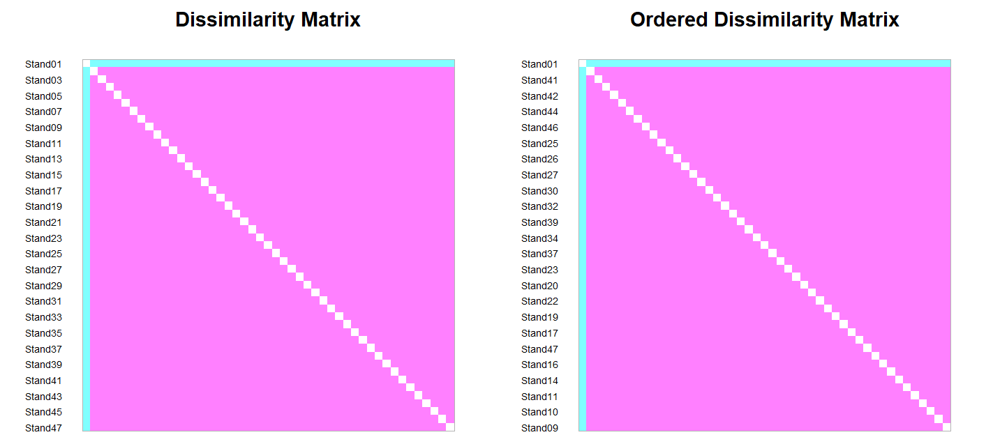
Bluer colors indicate pairs of plots that are far from one another, and pinker colors indicate pairs of plots that are closer to one another.  The left-hand image shows the stands as ordered in the distance matrix, while the right-hand image shows the stands after ordering them so that similar stands are grouped together.

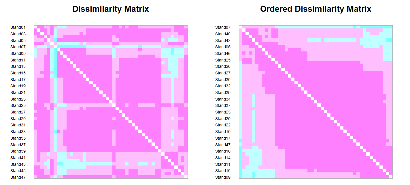
For comparison, here is the heat map based on the correct distances among stands:

coldiss(original.dis, byrank = FALSE)

The difference between these two distance matrices can also be viewed by viewing each distance matrix as a vector of numbers.  We’ll combine these together so that we can graph them below:

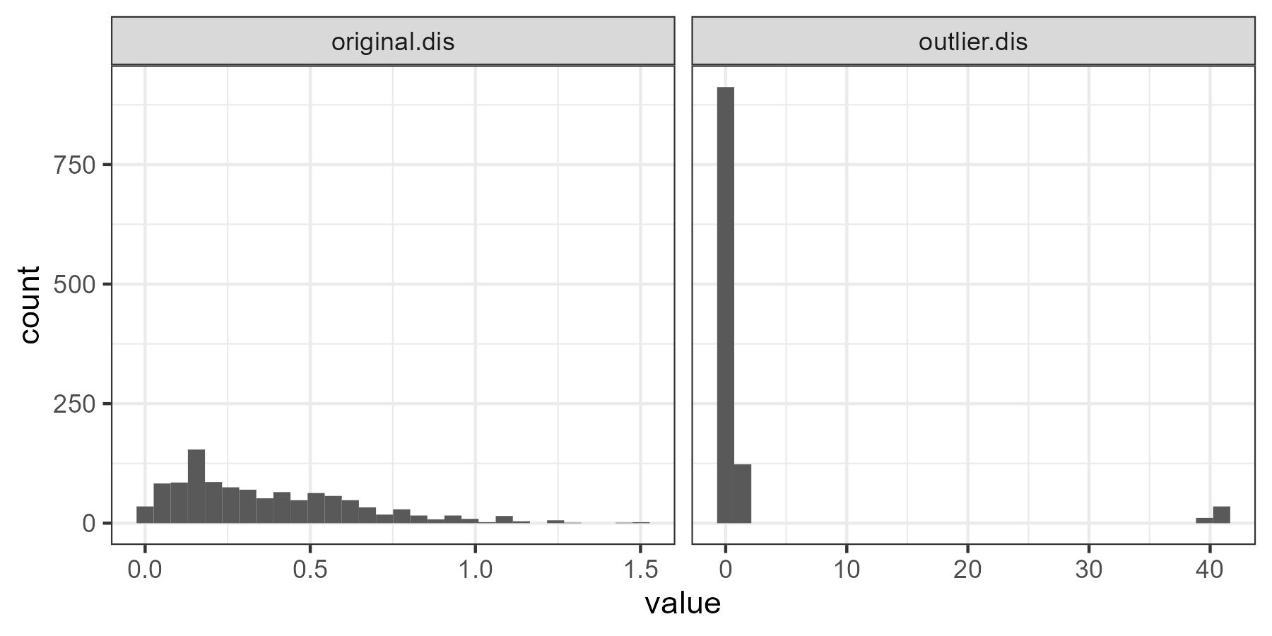
Dissimilarity Analysis (labdsv::disana())

The disana() function from labdsv provides a graphical and numerical summary of a distance matrix.  It produces a series of three graphs summarizing the distribution of values within the matrix:

1. Dissimilarity values, ranked from lowest to highest.  Do you understand why there are so many data points on this graph?  (hint: what is the formula for determining how many unique pairwise combinations there are?)
2. Minimum, mean, and maximum dissimilarity values for each sample unit.
3. Mean dissimilarity as a function of minimum dissimilarity.  Note that you are asked in the Console if you want to identify individual plots.  If you enter ‘Y’, the pointer changes to cross-hairs and you can click on data points in the graph.  When done, press ‘Esc’ or choose ‘Finish’ to break out of the plot ID routine.  The names of the points that you chose will be added to the graph.

The results of disana() can also be saved to an object.  This object is of class ‘list’.  It contains the minimum, mean, maximum dissimilarity of each plot to all others, as well as a vector identifying any samples selected in the last graph.  You can inspect the structure of this object using the str() function, and can also extract individual components for further analysis or use.

Applying this to our example:
outliers <- disana(outlier.dis)

To illustrate how the components of this object can be used, let’s duplicate the last plot created by disana() – the minimum dissimilarity compared to the minimum dissimilarity.

merge(outliers$min, outliers$mean, by = "row.names") |>
  rename(min = x, mean = y) |>
  ggplot(aes(x = min, y = mean)) +
    geom_point() +
theme_bw()

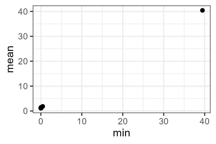
Note how strongly the outlier stands out from all of the others.

For comparison, apply disana() to the original distance matrix and then duplicate the above graphic.

Mahalanobis Distance

The Mahalanobis distance is a measure of how likely it is that an individual belongs to a group.  In Section 5.3, Manly & Navarro Alberto (2017) describe how this can be done – their script is available in the book’s online resources.  Several of the functions outlined in the ‘Common Distance Measures’ chapter can calculate Mahalanobis distances, but I haven’t investigated this fully.  In particular, the conventional Mahalanobis distance was developed for multivariate normal data but it would also be possible to modify this technique so it is applicable to other distributional forms, such as by calculating the distance between each plot and the centroid (‘center of mass’) of the rest of the sample units rather than the multivariate mean.

Jackson & Chen (2004) reported that a method based on the calculation of minimum volume ellipsoids worked better than Mahalanobis distances, though I haven’t seen (or looked for) a function to do this in R.  Another option is to write a function in which the mean distance from one sample unit to all others is calculated and compared to the mean distance among all other sample units.  If a sample unit is an outlier, the mean distance from it to the others will be larger than the mean distance among other sample units.

Conclusions

Multivariate outliers should be investigated further to see why they are outliers.  If a sample differs strongly from others in a single variable, does it reflect a data entry error that needs to be corrected?  If a sample differ from others with respect to multiple variables, was it perhaps assigned to the wrong group?  You as the investigator ultimately have to decide how to deal with outliers and whether or not to include them in your analyses.

References

Borcard, D., F. Gillet, and P. Legendre. 2018. Numerical ecology with R. 2nd edition. Springer, New York, NY.

Jackson, D.A., and Y. Chen. 2004. Robust principal component analysis and outlier detection with ecological data. Environmetrics 15:129-139.

Manly, B.F.J., and J.A. Navarro Alberto. 2017. Multivariate statistical methods: a primer. Fourth edition. CRC Press, Boca Raton, FL.

Zuur, A.F., E.N. Ieno, and C.S. Elphick. 2010. A protocol for data exploration to avoid common statistical problems. Methods in Ecology and Evolution 1:3-14.