
Classification
32 Discriminant Analysis
Learning Objectives
To assess how well observations have been classified into groups using linear methods (LDA) and distance-based methods (dbDA).
Key Packages
require(MASS, WeDiBaDis)
Introduction
Techniques such as cluster analysis are used to identify groups a posteriori based on a suite of correlated variables (i.e., multivariate data). This type of analysis is sometimes followed by an assessment of how well observations were classified into the identified groups, and how many were misclassified. This assessment is known as a discriminant analysis (DA) (aka canonical analysis or supervised classification). Williams (1983) notes that DA can be conducted for two reasons:
- Descriptive – to separate groups optimally on the basis of the measurement values
- Predictive – to predict the group to which an observation belongs, based on its measurement values
In these notes, I demonstrate linear and distance-based DA techniques.
- Linear discriminant analysis (LDA) is the most common method of DA. It is an eigenanalysis-based technique and therefore is appropriate for normally-distributed data.
- As implied by the name, distance-based discriminant analysis (Anderson & Robinson 2003) can be applied to any type of data, including community-level data and data types such as categorical variables that cannot be incorporated into LDA. Irigoien et al. (2016) describe how these techniques can be used in biology (e.g., morphometric analysis for species identification), ecology (e.g., niche separation by sympatric species), and medicine (e.g., diagnosis of diseases).
Linear Discriminant Analysis (LDA)
Theory
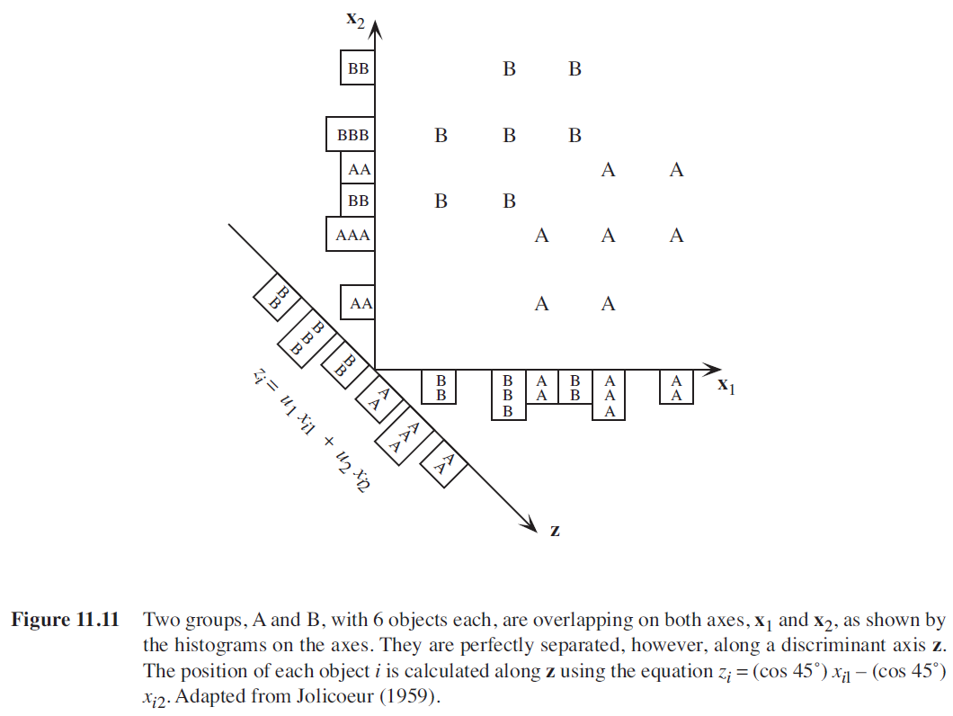
Rather than relating individual variables to group identity, LDA identifies the combination of variables that best discriminates (distinguishes) sample units from different groups. Combinations of variables can be more sensitive than individual variables. In the below figure (Figure 11.11 from Legendre & Legendre 2012), analyses that focus just on x1 or just on x2 cannot distinguish these groups (compare the histograms shown along the x1 and x2 axes). However, when x1 and x2 are combined into a new composite variable z, that variable clearly distinguishes the two groups (see histogram along the z axis).
LDA is an eigenanalysis technique (refer back to the chapter about matrix algebra if that term doesn’t sound familiar; we’ll discuss eigenanalysis in more detail when we focus on PCA) that also incorporates information about group identity. Conceptually, it can be thought of as a MANOVA in reverse:
| Explanatory (Independent) Variable(s) | Response (Dependent) Variable(s) | |
| MANOVA | Group Identity | Data |
| LDA | Data | Group Identity |
Given the similarity between LDA and MANOVA, it is perhaps unsurprising that LDA has the same assumptions with respect to multivariate normality, etc. It can be applied to data that satisfy these assumptions; environmental and similar types of data might meet these assumptions, but community-level data do not. It is important to keep in mind that it identifies linear combinations of variables.
For more information on LDA, see chapter 8 in Manly & Navarro Alberto (2017) and section 11.3 in Legendre & Legendre (2012).
Why Use LDA?
LDA has been used for various ecological applications, as described by McCune & Grace (2002, p. 205). Williams (1983) provides citations of some older ecological examples of LDA. Leva et al. (2009) provide an ecological example of how LDA might be applied. In their study, they measured a number of traits of the roots of eight grasses and then used LDA to classify observations to species on the basis of these traits. They also used cluster analysis and PCA to help understand the correlations between these traits and relationships among the species.
The most common reason to use LDA is to assess how well observations from different groups can be differentiated from one another on the basis of their measured responses. For example, the below dataset involves a bunch of measurements on a number of Darlingtonia plants. How well do these variables help us identify the site at which they were collected?
Here’s another potential application: suppose a field assistant measured another Darlingtonia plant but forgot to record the site they were working at. Their datasheet contains all of the measured variables except the site ID, so this plant isn’t included in our dataset. Can we use the relationships among the measured variables to predict which site the plant came from?
Example Dataset: Darlingtonia californica
We’ll illustrate LDA using detailed morphological measurements from 87 Darlingtonia californica (cobra lily; California pitcherplant) plants at four sites in southern Oregon. These data are from Table 12.1 of Gotelli & Ellison (2004), and are the same ones that we use to illustrate Principal Component Analysis (PCA).
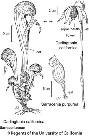
In this plant, leaves are modified into tubes that can hold liquid and trap insects. The 10 measured variables (and their units) are:
| Name | Type | Description | Units |
| height | Morphological | Plant height | mm |
| mouth.diam | Morphological | Diameter of the opening (mouth) of the tube | mm |
| tube.diam | Morphological | Diameter of the tube | mm |
| keel.diam | Morphological | Diameter of the keel | mm |
| wing1.length | Morphological | Length of one of the two wings in the fishtail appendage (in front of the opening to the tube) | mm |
| wing2.length | Morphological | Length of second of the two wings in the fishtail appendage (in front of the opening to the tube) | mm |
| wingsprea | Morphological | Length from tip of one wing to tip of second wing | mm |
| hoodmass.g | Biomass | Dry weight of hood | g |
| tubemass.g | Biomass | Dry weight of tube | g |
| wingmass.g | Biomass | Dry weight of fishtail appendage | g |
The datafile is available through the GitHub repository. We begin by importing the data.
darl <- read.csv("data/Darlingtonia_GE_Table12.1.csv")
The variables differ considerably in terms of the units in which they are measured, so it makes sense to normalize them (i.e., convert them to Z-scores) before analysis:
darl.data <- scale(darl[,3:ncol(darl)])
However, this is much less important for LDA than it is for PCA. To verify that the results of an LDA are not affected by this normalization, try running the below analyses using unscaled (raw) data from these Darlingtonia plants.
LDA in R (MASS::lda())
We will use the lda() function in the MASS package, though other options also exist. The usage of lda() is:
lda(x,
grouping,
prior = proportions,
tol = 1.0e-4,
method,
CV = FALSE,
nu,
…
)
The key arguments are:
x– the matrix or data frame containing the explanatory variables. This and the grouping argument could be replaced by a formula of the form
groups ~ x1 + x2 + .... Note that this formula is the opposite of that for an ANOVA – the grouping variable is the response here.grouping– a factor specifying the group that each observation belongs to.prior– prior probabilities of group membership. Default is to set probabilities equal to sample size (i.e., a group that contains more observations will have a higher prior probability).tol– tolerance to decide whether the matrix is singular (based on whether variance is smaller than tol^2). Default is 0.0001.method– how to calculate means and variances. Options:moment– standard approach (means and variances), and the default.mle– via maximum likelihood estimationmve– for a subset of the data that you specify (to exclude potential outliers)t– based on a t-distribution.
CV– whether to perform cross-validation or not. Default is to not (FALSE). Note that this argument is spelled with capital letters.nu– degrees of freedom (required ifmethod = “t”).
The resulting object includes several key components:
prior– The prior probabilities of class membership used. As noted above, the default is that these are proportional to the number of sample units in each group. See ‘Misclassifications’ section below for more details about this.means– The mean value of each variable in each group (be sure to note whether these are standardized or unstandardized).scaling– A matrix of coefficients (eigenvectors) of linear discriminant (LD) functions. Note that there is one fewer LD than there were groups in the dataset (because if you know that an observation doesn’t belong to one of these groups then it must belong to the last group). These are roughly analogous to the loadings produced in a PCA. Since we standardized our data before analysis, we can compare the LD coefficients directly among variables. Larger coefficients (either positive or negative) indicate variables that carry more weight with respect to that LD. The position of a given observation on a LD is calculated by matrix multiplying the measured values for each variable by the corresponding coefficients.- The proportion of variation explained by each LD function (eigenvalue). Note that these always sum to 1, and are always in descending order (i.e., the first always explains the most variation).
Applying lda() to the Darlingtonia Data
Let’s load the MASS package and then carry out an LDA of the Darlingtonia data:
library(MASS)
darl.da <- lda(x = darl.data, grouping = darl$site)
darl.da <- lda(darl$site ~ darl.data) # Equivalent
darl.da
Call:
lda(darl$site ~ darl.data)

Prior probabilities of groups:
       DG        HD       LEH       TJH
0.2873563 0.1379310 0.2873563 0.2873563

Group means:
    darl.dataheight darl.datamouth.diam darl.datatube.diam darl.datakeel.diam
DG       0.03228317          0.34960765        -0.64245369         -0.3566764
HD      -0.41879232         -1.37334175         0.93634832          1.3476695
LEH      0.22432324          0.25108333         0.23567347         -0.4189580
TJH     -0.05558610          0.05851306        -0.04266698          0.1287530
    darl.datawing1.length darl.datawing2.length darl.datawingsprea
DG              0.3998415             0.2997874         -0.2093847
HD             -0.8102232            -0.3184490         -0.1996899
LEH             0.5053448             0.3853959          0.6919511
TJH            -0.5162792            -0.5323277         -0.3867152
    darl.datahoodmass.g darl.datatubemass.g darl.datawingmass.g
DG            0.4424329          0.30195655          0.03566704
HD           -1.1498678         -1.05297022         -0.28283531
LEH          -0.1754338          0.07558687          0.23585050
TJH           0.2849374          0.12788229         -0.13575660

Coefficients of linear discriminants:
                              LD1        LD2         LD3
darl.dataheight        1.40966787  0.2250927 -0.03191844
darl.datamouth.diam   -0.76395010  0.6050286  0.45844178
darl.datatube.diam     0.82241013  0.1477133  0.43550979
darl.datakeel.diam    -0.17750124 -0.7506384 -0.35928102
darl.datawing1.length  0.34256319  1.3641048 -0.62743017
darl.datawing2.length -0.05359159 -0.5310177 -1.25761674
darl.datawingsprea     0.38527171  0.2508244  1.06471559
darl.datahoodmass.g   -0.20249906 -1.4065062  0.40370294
darl.datatubemass.g   -1.58283705  0.1424601 -0.06520404
darl.datawingmass.g    0.01278684  0.0834041  0.25153893

Proportion of trace:
   LD1    LD2    LD3
0.5264 0.3790 0.0946
You should be able to link parts of this output to the key components produced by lda() in its description above. Each piece can also be indexed or calculated separately, of course.
The prior probabilities here are simply the number of samples from a site divided by the total number of samples. They therefore have to sum to 1.
The coefficients of linear discriminants – an eigenvector – would be multiplied by the corresponding variables to produce a score an individual observation on a particular LD. To view just the matrix of coefficients for each LD function:
darl.da$scaling %>% round(3)
                         LD1    LD2    LD3
darl.dataheight        1.410  0.225 -0.032
darl.datamouth.diam   -0.764  0.605  0.458
darl.datatube.diam     0.822  0.148  0.436
darl.datakeel.diam    -0.178 -0.751 -0.359
darl.datawing1.length  0.343  1.364 -0.627
darl.datawing2.length -0.054 -0.531 -1.258
darl.datawingsprea     0.385  0.251  1.065
darl.datahoodmass.g   -0.202 -1.407  0.404
darl.datatubemass.g   -1.583  0.142 -0.065
darl.datawingmass.g    0.013  0.083  0.252
The larger these values are (in absolute terms), the more important that variable is for determining the location of a plant along that LD. For example, plant height is much more important for LD1 than for LD2 or LD3.
The values labeled as ‘proportion of trace’ on the screen are calculated as:
(darl.da$svd^2/sum(darl.da$svd^2)) %>% round(3)
0.526 0.379 0.095These proportions – the eigenvalues – are associated with the LDs, and are always in descending order (LD1 > LD2 > LD3 > …). They also sum to 1. The first LD is the important important for discriminating between the groups, and LD3 is least important of these three.
Plotting a LDA
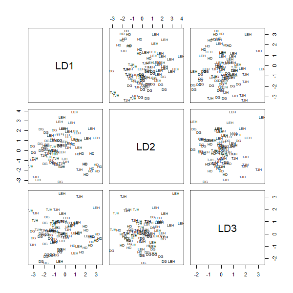
To graph all pairwise combinations of LDs:
plot(darl.da) #pairs(darl.da) is equivalent
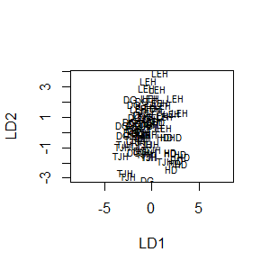
We can add the ‘dimen’ argument to specify how many LDs to plot. To plot LD1 vs LD2:
plot(darl.da, dimen = 2)
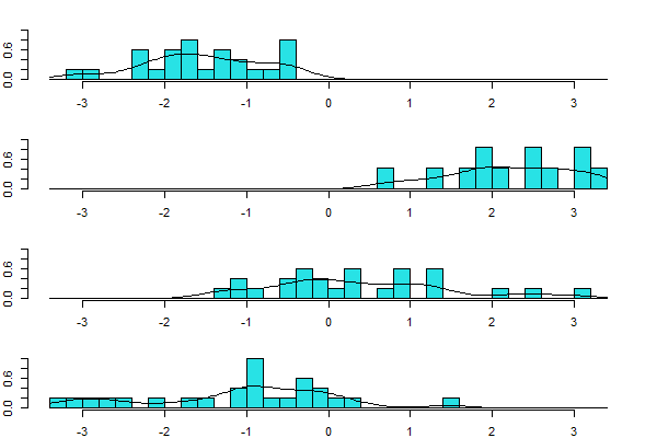
To plot just LD1 for each group:
plot(darl.da, dimen = 1, type = "both")
The ‘type’ argument here specifies whether to graph “histogram“, “density“, or “both“.
Misclassifications
How well were we able to predict which site an individual came from on the basis of these morphological data? We can use the predict() function to predict the group that each individual belongs to:
darl.predict <- predict(darl.da)
This function returns three components:
class– The predicted group identity of each observation.posterior– The posterior probability that each observation belongs to each of the four sites. Note that larger values are better, and the plant is predicted to belong to the site in which it has the largest posterior value. For any observation, the posterior probabilities of the different groups will sum to 1.x– The scores of each observation for each LD.
For example, here are the predicted group identities of the first few observations:
head(darl.predict$class)
[1] DG  TJH LEH TJH DG  TJH
Levels: DG HD LEH TJH
The first observation was predicted to belong to site DG, the second to site TJH, etc.
How well were observations classified according to site? We can summarize this in a cross-classification table (aka confusion matrix), the results of which are shown below:
darl.table <- table(darl$site, darl.predict$class)

darl.table
      DG HD LEH TJH
  DG  18  0   2   5
  HD   0 11   1   0
  LEH  3  0  21   1
  TJH  2  0   3  20
The rows in this table correspond to the true classification, and the columns to the predicted classification from the DA. The row totals (not shown) are the actual numbers of observations in each group. Values along the diagonal are correctly predicted; all others are misclassified. The percentage of observations that were correctly classified is:
sum(diag(darl.table))/sum(darl.table) * 100
So, about 80% of observations were correctly classified. You could also index this calculation to figure out this percentage separately for each site.
Prior Probabilities
One important aspect of a DA is the decision of what prior probabilities to use. These probabilities are weights in the calculations of a DA: the higher the probability, the more weight a group is given. We often assume that the prior probabilities are either i) equal among groups, or ii) proportional to sample sizes. Unless otherwise specified, the lda() function assumes that prior probabilities are equal to sample sizes.
The prior probabilities can alter the likelihood and direction of misclassification. Whether the direction matters depends on the situation. McCune & Grace (2002, p. 209-210) give an example in which the prior probabilities altered the classification of sites as goshawk nesting habitat or not. These differences could easily affect land management. More significant consequences can occur in medical studies: for example, consider the difference between misclassifications that predict someone has cancer when they don’t, and misclassifications that predict they don’t have cancer when they actually do. Which would you prefer?
Cross-Validation
The above confusion matrix permitted us to assess the results of a DA by comparing them against the observed data. Data can also be cross-validated in various ways:
- Jackknifing. In
lda(), this can be done by adding the ‘CV = TRUE’ argument to the function. Jackknifing involves the following steps:- omit one observation from dataset
- analyze reduced dataset
- use results to classify the omitted observation
- repeat for next observation in dataset
- Reserving a subset of the data as an independent validation dataset. These data are not used in the initial analysis, but are used to assess how well the classification works. This is only feasible if the dataset is large.
- Collect new data and use DA to classify it (though there needs to be some way to independently verify that they are classified correctly).
Jackknifing the darl data:
darl.da.CV <- lda(darl$site ~ darl.data, CV = TRUE)
We can use a confusion matrix to compare the results of the cross-validated LDA with the original classification (or with the results of the LDA without cross-validation).
table(darl$site, darl.da.CV$class)
      DG HD LEH TJH
  DG  17  1   2   5
  HD   0 10   2   0
  LEH  4  1  18   2
  TJH  3  1   3  18
With cross-validations, the accuracy has declined to 72% (ensure you understand how this was calculated).
We can also compare the posterior probabilities produced via jackknifing with those predicted from the original LDA based on all data. For the first observation (and rounding probabilities to 3 decimal places:
darl.da.CV$posterior[1,] %>% round(3)
   DG    HD   LEH   TJH
0.875 0.000 0.000 0.124
darl.predict$posterior[1,] %>% round(3)
   DG    HD   LEH   TJH
0.772 0.000 0.000 0.228
To compare all observations, we might focus on the differences between the probabilities:
(darl.da.CV$posterior – darl.predict$posterior) %>%
round(3) %>%
head()
     DG    HD   LEH    TJH
1 0.104 0.000 0.000 -0.104
2 0.086 0.000 0.021 -0.107
3 0.002 0.004 0.060 -0.066
4 0.052 0.000 0.002 -0.054
5 0.074 0.000 0.009 -0.084
6 0.057 0.000 0.001 -0.058
Note that a reduced posterior probability for one or more groups must be accompanied by an increased posterior probability in one or more other groups. Large differences indicate observations that strongly affect the LDA; the result of the jackknifing differs considerably when they are omitted.
Key Takeaways
Cross-validation is important for assessing how well the products of a LDA can classify independent observations.
Distance-based Discriminant Analysis (WeDiBaDis::WDBdisc())
Anderson & Robinson (2003) present an alternative method for conducting a DA on the basis of a distance matrix. Since any distance measure can be used to calculate the distance matrix, they suggest this method can be used for community-level data. This appears to involve using metric multidimensional scaling to reduce the dimensionality of the data and express it in Euclidean units, followed by a LDA on the locations of the sample units in the reduced ordination space.
Irigoien et al. (2016) provide a package, WeDiBaDis (Weighted Distance Based Discriminant Analysis) that provides this functionality. It is available through their GitHub page:
library(devtools)
install_github("ItziarI/WeDiBaDis")
Load the package once it’s installed:
library(WeDiBaDis)
The usage of the key function, WDBdisc(), is as follows:
WDBdisc(data,
datatype,
classcol = 1,
new.ind = NULL,
distance = "euclidean",
method,
type
)
The key arguments are:
data– a data matrix or distance matrix, with a column containing the class labels (grouping factor). By default, the class labels are assigned to be in the first column; this is set by theclasscolargument.datatype– ‘m’ if data are a data matrix, ‘d’ if data are a distance matrix.classcol– column number in which actual classification is coded. Default is the first column.new.ind– whether or not there are new individuals to be classified.distance– type of distance measure to be used if data is a data matrix. Options areeuclidean(default),correlation,Bhattacharyya,Gower,Mahalanobis,BrayCurtis,Orloci,Hellinger, andPrevosti.method– whether to conduct distance-based DA (DB) or weighted distance-based DA (WDB). I haven’t delved into the basis of the weighting, but it can be helpful if the sample sizes differ among groups.
The output includes a number of elements:
conf– the confusion matrix relating the actual classification to the classification as predicted by the explanatory variables. This is the same type of table that we calculated above.pred– predicted class for observations that did not have an actual classification, if any were included.
A visual representation of the confusion matrix can be seen via the plot() function.
The summary() function can be applied to the output and produces additional information:
- Total correct classification: the sum of the diagonals of the confusion matrix divided by the total number of observations (as calculated above).
- Generalized squared correlation: ranges from 0 to 1. A value of 0 means that there is at least one class in which no units are classified.
- Cohen’s Kappa coefficient: a measure of the agreement of classification to the true class. Irigoien et al. (2016) provide the following rules of thumb for interpreting it:
- < 0: less than chance agreement
- 0.01-0.20: slight agreement
- 0.21-0.40: fair agreement
- 0.41-0.60: moderate agreement
- 0.61-0.80: substantial agreement
- 0.81-0.99: almost perfect agreement
- Sensitivity (or recall), for each class. The number of observations correctly predicted to belong to a given class, as a percentage of the total number of observations in that class.
- Precision (positive predictive value), for each class. Probability that a classification in this class is correct.
- Specificity, for each class. A measure of the ability to correctly exclude an observation from this class when it really belongs to another class.
- F1-score, for each class. Calculated based on sensitivity and precision.
The sensitivity, precision, and specificity can also be graphed by plotting the output of this summary function.
Applying WDBdisc() to the Darlingtonia data
Note that this function requires the data in a specific format that contains both the response (classification) and the explanatory variables. In this case, we’ll provide the explanatory variables and allow the function to apply the Euclidean distance matrix to it (with other datasets, we could specify a different distance measure or provide a matrix of distances). And, since the number of observations differs among sites, we’ll use the weighted DA.
darl.WDB <- cbind(darl$site, darl.data)
darl.dbDA <- WDBdisc(data = darl.WDB,

datatype = "m",
classcol = 1,

method = "WDB")
summary(darl.dbDA)
Discriminant method:
------ Leave-one-out confusion matrix: ------
     Predicted
Real  DG HD LEH TJH
  DG  11  0   8   6
  HD   0 10   0   2
  LEH  0  3  20   2
  TJH  3  6   6  10

Total correct classification:  58.62 %

Generalized squared correlation:  0.2632

Cohen's Kappa coefficient:  0.4447793

Sensitivity for each class:
   DG    HD   LEH   TJH
44.00 83.33 80.00 40.00

Predictive value for each class:
   DG    HD   LEH   TJH
78.57 52.63 58.82 50.00

Specificity for each class:
   DG    HD   LEH   TJH
64.52 54.67 50.00 66.13

F1-score for each class:
   DG    HD   LEH   TJH
56.41 64.52 67.80 44.44
------ ------ ------ ------ ------ ------

No predicted individuals
Note that the confusion matrix is a leave-one-out confusion matrix, which means that jackknifing has automatically been performed.
Just under 60% of the observations are being correctly classified. Cohen’s Kappa indicates moderate agreement between the actual classification and the classifications based on these variables. Observations at the HD and LH sites are particularly well classified.
To see a visualization of the confusion matrix:
plot(darl.dbDA)
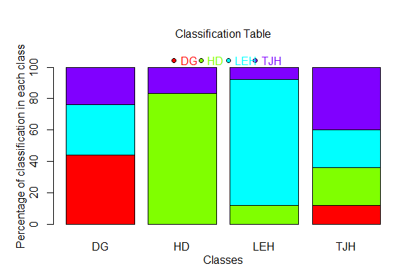
The bars in this plot are the actual sites (labeled ‘Classes’). The colors also distinguish sites. The portion of a bar that is the same color as the label beneath the bar is the plants that were correctly classified to the site that they actually came from. Other colors within a bar indicate the other sites to which plants from that site were classified. For example, most of the plants from site LEH (light blue color) were correctly classified, and none of the plants from this site were classified as belonging to site HD.
Finally, the summary() output can also be plotted:
plot(summary(darl.dbDA))

This summarizes the sensitivity, positive predicted value, and specificity for each group.
Key Takeaways
Distance-based discriminant analysis provides a method for classifying observations in situations where assumptions about linearity are not appropriate.
Conclusions
Discriminant analysis is an important tool for understanding differences among groups and using those differences to predict (classify) the group to which other samples belong. It is common for example in medical statistics in terms of evaluating the accuracy of diagnoses.
The medical context is also helpful for recognizing that there may be dramatically different consequences for different types of misclassification – for example, the distinction between classifying someone as having a disease when they actually don’t (false positive) and classifying someone as not having a disease when they actually do (false negative) (Irigoien et al. 2016).
References
Anderson, M.J., and J. Robinson. 2003. Generalized discriminant analysis based on distances. Australian and New Zealand Journal of Statistics 45:301-318.
Gotelli, N.J., and A.M. Ellison. 2004. A primer of ecological statistics. Sinauer, Sunderland, MA.
Irigoien, I., F. Mestres, and C. Arenas. 2016. Weighted distance based discriminant analysis: the R package WeDiBaDis. The R Journal 8:434-450.
Legendre, P., and L. Legendre. 2012. Numerical ecology. Third English edition. Elsevier, Amsterdam, The Netherlands.
Leva, P.E., M.R. Aguiar, and M. Oesterheld. 2009. Underground ecology in a Patagonian steppe: root traits permit identification of graminoid species and classification into functional types. Journal of Arid Environments 73:428-434.
Manly, B.F.J., and J.A. Navarro Alberto. 2017. Multivariate statistical methods: a primer. Fourth edition. CRC Press, Boca Raton, FL.
McCune, B., and J.B. Grace. 2002. Analysis of ecological communities. MjM Software Design, Gleneden Beach, OR.
McKenna Jr., J.E. 2003. An enhanced cluster analysis program with bootstrap significance testing for ecological community analysis. Environmental Modelling & Software 18:205-220.
Williams, B.K. 1983. Some observations on the use of discriminant analysis in ecology. Ecology 64:1283-1291.
Media Attributions
- Legendre.Legendre.2012_Figure.11.11
- Darlingtonia.californica_Jepson
- LDA.pairs
- LDA.2D
- LDA.1D
- dbDA.classification.table
- dbDA.summary
