
Foundational Concepts
7 Relativizations
Learning Objectives
To consider how relativizations / standardizations relate to the research questions being addressed.
To illustrate how to relativize data in R.
Readings
Fox (2013 blogpost)
Key Packages
require(vegan)
Relativizations / Standardizations
A relativization or standardization is a transformation that is affected by other elements in the matrix. Another way to think of this is that the action taken on an individual element would be different if you consider it alone or as part of a set of elements.
Relativizations can be applied to rows (sample units), columns (variables), or both. For example, relativizing a data frame by columns will mean that each element within a given column is adjusted based on the values of other elements in that same column.
Relativizations can also be applied in series – for example, relativizing elements on a row-by-row basis and then further relativizing those relativized elements on a column-by-column basis. See the Wisconsin standardization below as one example of this.
Relativizations are particularly important in some situations:
- To permit equitable comparisons when variables are measured in different units. For example, the metadata of our sample dataset indicates that tree abundance is expressed as basal area (ft2/acre) whereas the abundance of other taxa is expressed as percent cover. Furthermore, note that basal area has no upper bound whereas percent cover cannot exceed 100% for a species. It therefore would not make sense to directly compare the absolute abundance of a tree species to the absolute abundance of another type of species.
- To permit equitable comparisons when variables are expressed on different scales. Imagine a study in which the heights of trees and grasses were measured. The trees might be measured in m and the grasses in cm. Simply expressing them on the same scale (e.g., cm) would mean that the much larger numerical values for trees would overwhelm the smaller value for grasses.
- To explore questions about relative differences, as described below.
The relativizations described below are often based on a single variable, but another approach is to relativize on the basis of another variable. For example, in wildlife studies abundance is commonly divided by sampling effort to account for differences in sampling effort (Hopkins & Kennedy 2004). This was also evident in the medical trial reported below, where the number of cases was expressed per 10,000 women.
We’ll talk about distance measures soon, but for now I’ll note that some are based on absolute differences between sample units and others on relative differences between sample units. Many distance measures based on absolute differences become mathematically equivalent following relativization.
Relativizations
Relativizations are conditional: the change in one element depends on which other elements are present in the object.
Theory
Analyses based on absolute values and on relative values address different questions. Imagine a study in which you capture and count the animals in an area. What hypotheses might be tested if you analyze the number of raccoons captured (an absolute value)? What about if you analyze the proportion of all animals captured that were raccoons (a relative value)?
The below image nicely illustrates the ways that absolute and relative effects can relate to one another, including that one effect can be a cost (negative) while the other is a benefit (positive)!
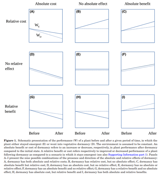
Grace (1995) provides an example of how a dataset can be used to answer one set of questions based on absolute values and another set of questions based on relative values (see Freckleton et al. (2009) for more of this conversation). And, Fox (2013) provides some nice examples of the difference between absolute and relative fitness.
The fact that absolute and relative values can answer different questions can be used to mislead. As an example of the latter, Yates (2019) notes that medical trials commonly report positive outcomes “in relative terms, to maximize their perceived benefit” but side effects “in absolute terms in an attempt to minimize the appearance of their risk” (p. 133). He illustrates this with a study of a breast cancer treatment, in which the drug reduced the occurrence of breast cancer but was also associated with increased occurrence of uterine cancer. I’ve summarized the data below, highlighting the statistics that were used to interpret the results. Can you see how this can be misleading?
| Treatment | Cases Per 10,000 Women | |
| Breast Cancer | Uterine Cancer | |
| Drug | 133 | 23 |
| Placebo | 261 | 9 |
| Relative Change due to Drug (difference between Drug and Placebo, divided by Placebo) | -49% | 156% |
How to decide what to do? As McCune & Grace (2002, p. 70) note, “there is no right or wrong answer to the question of whether to relativize until one specifies the question and examines the properties of the data”.
Absolute and Relative Effects
Knowing the direction and magnitude of an absolute effect does not necessarily tell you the direction and magnitude of a corresponding relative effect. It is possible for them to respond similarly, or for one to be positive and the other to be neutral or negative.
Types of Relativizations
I summarize some common relativizations here.
Normalize (Adjust to Standard Deviate)
If variables are normally distributed, they can be standardized into Z-scores:
[latex]Z = \frac {Y_{i} - \bar Y} {s}[/latex]
where [latex]{Y_{i}}[/latex] is the value of Y in the ith sample unit, [latex]{\bar Y}[/latex] is the mean value of Y, and [latex]{s}[/latex] is the standard deviation of Y.
After normalization, the values for a variable are expressed in units of how many standard deviations they are from the mean (negative if below the mean, positive if above the mean). As a result, this relativization can permit equitable comparisons among variables even if they were measured in very different units.
This is commonly applied to columns of normally-distributed data. This relativization is generally not applied to species abundances but is very reasonable for other response variables and for some explanatory variables.
It rarely makes sense to apply this relativization to rows.
Relativize by Maximum
Set maximum value to 1 and calculate all other elements as a proportion between 0 and 1. This is commonly applied to the columns (species) of a species abundance matrix or to other variables where zero is a reasonable expectation for a minimum value.
When applied to species abundance data, this allows species to contribute equally to differences between plots. Assuming that two species were absent from some plots, and thus have zero as their minimum, their relativized values will span the same range even if they differed greatly in abundance.
Relativize by Range
Set maximum value to 1 and minimum value to 0, and calculate all other elements as proportions between these two values.
This relativization is similar to relativizing by maxima but is useful for variables that do not have zero as the expected minimum value. For example, it would be more appropriate to relativize the latitude of each plot (Oak$LatAppx or Oak_explan$LatAppx) by range than by maxima. Do you see why this is the case? Try calculating and comparing the two approaches!
Adjust to Mean
Subtract row or column mean from each element. An element that was smaller than the mean will produce a negative number, while an element that was larger than the mean will produce a positive number.
This is the numerator of the Z-score calculation used to normalize data above. However, it does not change the units in which variables are measured.
Binary
If binary decisions are made on the basis of a static value, such as ‘greater than zero’, then they are transformations as discussed in that chapter. However, if the threshold value depends on other elements in the matrix, then a binary adjustment is a relativization. For example, one plausible relativization is to set all values smaller than the median to 0 and all values larger than the median to 1. Since the median depends on other values in the matrix, the outcome for any element depends on which other elements are included in the dataset.
Weight by Ubiquity / Relativize by Total
Calculate value in each element as a proportion of the total of all values.
This is commonly applied to the rows (sample units) of a species abundance matrix. The resulting data equalizes the contribution of plots: the relativized data sum to 1 for every plot regardless of how much plots differed in total abundance. Note that it only makes sense to apply this to a set of values where the sum of those values is meaningful.
Sometimes it makes sense to apply this to a subset of the variables. For example, if the explanatory variables include depths of different soil horizons, you could relativize each horizon as a proportion of the total soil depth.
It rarely makes sense to apply this relativization to columns. To do so, the sum of the values in the column would have to be a meaningful value.
Common Relativizations
The most common relativizations are:
- Relativizing each column by its maximum or range or, if normally distributed, by converting it to a Z-score. These approaches equalize the importance of each column by accounting for differences in unit, scale, etc.
- Relativizing each row by its total. This equalizes the contribution of each row by adjusting for differences in total.
Will Relativization Make a Difference?
McCune & Grace (2002, p.70) note that the degree of variability in row or column totals can be used to assess whether relativization will have much of an effect. They are referring here to data that have been measured in the same units for all variables (columns) in all sample units (rows). In other words, it needs to make sense to compare row or column totals.
McCune & Grace express the degree of variability by the coefficient of variation (CV) of the row or column totals. The CV is the ratio of the standard deviation of a variable to its mean, multiplied by 100 to express it as a percentage. They propose the following benchmarks:
| CV (%) | Magnitude |
| < 50 | Small |
| 50-100 | Moderate |
| 100-300 | Large |
| > 300 | Very large |
The predicted effect of relativization is directly related to the magnitude of the CV: relativization by columns will have a greater effect if there is very large variation among the columns than if there is small variation among them. However, please note that these are only rules of thumb. Depending on your objectives, it may make sense to relativize even if the CV is small or to not relativize even if the CV is very large.
Row and column totals can be calculated using the rowSums() and colSums() functions. We can use these to calculate the CV.
We’ll illustrate this with our oak plant community dataset. To begin, we open the R project, load the data, and create separate objects for the response and explanatory data:
Oak <- read.csv("data/Oak_data_47x216.csv", header = TRUE, row.names = 1)
Oak_species <- read.csv("data/Oak_species_189x5.csv", header = TRUE)
Oak_abund <- Oak[ , colnames(Oak) %in% Oak_species$SpeciesCode]
Oak_explan <- Oak[ , ! colnames(Oak) %in% Oak_species$SpeciesCode]
See the ‘Loading Data‘ chapter if you do not understand what these actions accomplished.
Now, let’s calculate the CV among row totals:
100 * sd(rowSums(Oak_abund)) / mean(rowSums(Oak_abund)) # CV of row (plot) totals
Aside: A Simple Function to Calculate Coefficient of Variation
Note that we call rowSums(Oak_abund) twice in the above calculation of the CV. Adapting this for a different variable can therefore be error prone – for example, if we want to apply it to columns we might accidentally forget to change one of these calls to colSums(Oak_abund). Importantly, the code would still execute but the resulting numbers would be nonsensical.
An alternative is to create a function in which the repeated object is only specified once. To do so, we will replace the repeated object by a single argument:
CV <- function(x) { 100 * sd(x) / mean(x) }
This provides an opportunity to highlight some basic points about writing functions:
- Functions are created using the
function()function, and are assigned to an object name – in this case, ‘CV’. - The
function()function should include any arguments that you want to be able to specify while executing the function. In this case, we only have the argumentx, which is the object for which we want to calculate the standard deviation and mean. Within the function, we specify this argument wherever we want it to be replaced by the specified object when the function is executed. - The
function()function can also include any arguments that we want to be able to specify but for which we also want predefined default values. This example doesn’t have any such arguments, but they would take the form ‘argument = default’. - The {squiggly brackets} denote the beginning and end of the function; in this case it is only one line long. Other functions can span tens or hundreds of lines of code.
- Functions are assigned to an object name, and called using that name.
Applying our new CV() function:
CV(x = rowSums(Oak_abund)) # CV of plot totals
CV(x = colSums(Oak_abund)) # CV of species totals
This function can be used with any data, not just the row and column sums that we are focusing on here. For example:
CV(x = Oak_explan$Elev.m) # CV of plot elevations
Again, the advantage of a function is that all of the operations specified in the function are carried out every time it is called.
If you include the code for a function near the beginning of your script, it will be loaded each time you run your script, and available for use later in the script.
Applications in R
In R, there are several functions that can be used to relativize data. Some are applied to rows or columns by default – these are generally reasonable defaults, but necessary to be aware of.
apply()
The apply() function can be used to apply many functions to a matrix. The usage of this function is:
apply(X, MARGIN, FUN, ..., simplify = TRUE)
The key arguments are:
X– the matrix to be analyzedMARGIN– whether to apply the function to rows (1), columns (2), or both (c(1,2))FUN– the function to be applied
For example, we could use this function to calculate the species richness of each stand:
apply(X = Oak_abund > 0, MARGIN = 1, FUN = sum)
Note that we have incorporated some indexing into this function. Do you understand what this indexing did?
What would we be calculating if we switched the margin from 1 to 2?
scale() and sweep()
The scale() function centers and/or scales (i.e., normalizes) a matrix. Its usage is:
scale(x, center = TRUE, scale = TRUE)
The key arguments are:
x– the data matrixcenter– Subtract a specified value from each element in a columncenter = TRUE– subtract column mean. This is the default.center = FALSE– no centering done
scale– divide each element in a column by a valuescale = TRUE– divide by root mean square (standard deviation). This is the default.scale = FALSE– no scaling done
Note that centering always precedes scaling. If the default values are accepted, this normalizes each column.
In comparison, the sweep() function adjusts data on the basis of a summary statistic. This sounds and is generic – centering is a specific example in which the data are adjusted by subtracting the mean value. No scaling is involved.
For example, imagine that we want to express the abundance of species relative to their median values. You can verify that the following functions are identical:
Quga <- Oak_abund[ , c("Quga.s", "Quga.t")]
scale(x = Quga, center = apply(Quga, 2, median), scale = FALSE)
sweep(Quga, 2, apply(Quga, 2, median))(note that I restricted attention here to the two oak taxa simply for convenience when comparing them visually. Both functions could equivalently be applied to the entire data matrix).
vegan::decostand()
The decostand() function is a versatile means of relativizing (standardizing) data. Its usage is:
decostand(x, method, MARGIN, range.global, logbase = 2, na.rm = FALSE, ...)
The key arguments are:
x– the data frame or matrix to be relativizedmethod– relativization / standardization method to be applied. Each method has a default margin but can also be applied to the other one. I’ve highlighted those that are particularly useful as noted above.total– divide by margin total. By default, applied to rows.max– divide by margin maximum. This equalizes the contribution of each species in the matrix. By default, applied to columns.frequency– divide by margin maximum and then multiple by the number of non-zero elements so that the average of the non-zero entries is one. By default, applied to columns.normalize– make margin sum of squares equal to one. By default, applied to rows. Note that this is not the same as the normalizing that is discussed above.range– convert values to range from 0 to 1. By default, applied to columns.rank– convert abundance values to increasing ranks – in other words, the most abundant species will have the largest rank. Zeroes are left unchanged. By default, applied to rows.rrank–rank, relativized so that the highest rank is 1. By default, applied to rows.standardize– normalize data by converting it to Z-scores (i.e., mean = 0, variance = 1). Intended for normally distributed data. By default, applied to columns.pa– convert to presence/absence (1 or 0, respectively).chi.square– Divide by row sums and square root of column sums, and adjust for square root of matrix total. Can be problematic; we’ll discuss this in the context of correspondence analysis. By default, applied to rows.hellinger– square root oftotalmethod. By default, applied to rows.log– adjusts values based on a log (specified bylogbase). Values greater than zero are log-transformed, while zeroes are left unchanged. Note, therefore, that this is not a simple log transformation; see help for details.alr– additive log ratio. Commonly used with pH and other chemistry measurements.clr– centered log ratio. Commonly used in microbial ecology.rclr– robust centered log ratio.
MARGIN– whether to apply to rows (MARGIN = 1) or columns (MARGIN = 2). Each method has a default margin – explained in the ‘Details’ section of the help file – so this only has to be included if you want to apply the method to the non-default margin.na.rm– whether to ignore missing values
As an example, let’s relativize elevations by their range:
decostand(x = Oak_explan$Elev.m, method = "range")
In this case, the relativization was applied to one variable. Applying it to the entire dataframe is simply a matter of indexing, and of course making sure that decostand() is being applied to the correct margin. If we want to relativize our response data by the maximum of each species (column):
Oak_abund_max <- decostand(x = Oak_abund, method = "max")
vegan::wisconsin()
When working with species abundance data, a common approach is to standardize each species by its maximum, and then each site by its total. This double standardization is known as a Wisconsin standardization as it was first applied to data collected in that state.
Wisconsin standardization is simply done using the wisconsin() function:
Oak_abund_stand1 <- wisconsin(Oak_abund)
Verify that this is identical to the result of two calls to decostand(), first standardizing columns by their maxima and then rows by their totals:
Oak_abund_stand2 <- decostand(decostand(Oak_abund, "max"), "total") # nested functions
Oak_abund_stand2 <- Oak_abund |> decostand("max") |> decostand("total") # piped
Concluding Thoughts
Decisions about how to adjust data – including whether and which variables to relativize – can strongly affect the conclusions of subsequent analyses. Relativizations can be made to both response variables and explanatory variables. Most of the techniques that we are using in this course make minimal statistical assumptions, which means that adjustments do not have to be made for statistical reasons but rather can focus on the ecological questions of interest.
With species data, several types of standardization are common, depending on the objectives of the study. Some studies will not do any standardization, some will standardize columns only, some will standardize rows only, and some will standardize both rows and columns.
Relativizing by row may be appropriate for a full matrix or for appropriate subsets of the data. For example, it would not be appropriate to relativize by rows if the columns of interest were not logically related to one another (e.g., elevation, soil depth, aspect).
Relativizing by column can be particularly helpful when variables have not been measured on the same scale but want to be given equal weight. This is true for both response and explanatory variables.
Actions such as deleting rare species, transforming data, and relativizing data should be done through scripts, not through permanent changes to the raw data file. Scripting these actions ensures flexibility to try other adjustments, skip them entirely, etc.
Sometimes answering our ecological questions require a series of adjustments. The order of adjustments can affect the resulting data. See this appendix for guidance about the order in which to conduct data adjustments. For example, in one study (Mitchell et al. 2017) we analyzed plant community structure. Our raw data was a plot x species matrix where the elements were the abundance of each species in each plot in 2002. Our workflow included a number of steps:
- Summed the abundances of all species on a row-by-row basis to yield total cover.
- Transformed the abundances to presence/absence data, and then summed those data on a row-by-row basis to yield species richness.
- Grouped species by their functional group, and calculated the cover for each functional group. Then, we relativized the abundances by row totals (so, each row summed to 1), and calculated the proportion of the cover accounted for by each functional group. Thus, we were focusing on the relative abundance of these functional groups. We did not analyze absolute abundances.
- Combined these data with a similar plot x species matrix of the same plots in 1989 to determine how much composition had changed during this period. To combine data from these two years, we had to resolve taxonomic differences between years. We also elected to delete rare species. After these adjustments, we calculated the compositional change from 1989 to 2002 as the Bray-Curtis dissimilarity (one of the distance measures we’ll discuss soon) between the two years.
Which Adjustments to Make, and in What Order?
A series of adjustments are often required to organize the data in a way that permits our questions to be answered. Think carefully through which adjustments to make and in which order to make them – these decisions can affect the conclusions of analyses.
References
Fox, J. 2013. Do ecologists ever confuse absolute and relative fitness? https://dynamicecology.wordpress.com/2013/09/24/dont-confuse-absolute-and-relative-fitness/
Freckleton, R.P., A.R. Watkinson, and M. Rees. 2009. Measuring the importance of competition in plant communities. Journal of Ecology 97:379-384.
Grace, J.B. 1995. On the measurement of plant competition intensity. Ecology 76:305-308.
Hopkins, H.L., and M.L. Kennedy. 2004. An assessment of indices of relative and absolute abundance for monitoring populations of small mammals. Wildlife Society Bulletin 32:1289-1296.
Hurskainen, S., K. Alahuhta, H. Hens, A. Jäkäläniemi, T. Kull, R.P. Shefferson, and J. Tuomi. 2018. Vegetative dormancy in orchids incurs absolute and relative demographic costs in large but not in small plants. Botanical Journal of the Linnean Society 188:426-437.
McCune, B., and J.B. Grace. 2002. Analysis of ecological communities. MjM Software Design, Gleneden Beach, OR.
Mitchell, R.M., J.D. Bakker, J.B. Vincent, and G.M. Davies. 2017. Relative importance of abiotic, biotic, and disturbance drivers of plant community structure in the sagebrush steppe. Ecological Applications 27:756-768.
Yates, K. 2019. The Math of Life & Death: 7 Mathematical Principles That Shape Our Lives. Scribner, New York, NY.
Media Attributions
- Hurskainen.et.al.2018_Figure1
