
Group Comparisons
26 Restricting Permutations
Learning Objectives
To understand how to replicate analyses by restricting the set of permutations used.
To demonstrate how to conduct permutation tests of complex designs in R.
Readings
Recommended: Anderson & ter Braak (2003).
Key Packages
require(vegan, permute)
Introduction
The purpose of this chapter is to illustrate how to restrict permutations. This can be necessary for complex designs. Exactly how permutations need to be restricted will depend on the nature of your experimental design. While demonstrating a complex analysis, we will capitalize on the fact that a conventional ANOVA corresponds to a PERMANOVA of a univariate response with Euclidean distances.
In the notes that follow, I refer specifically to vegan::adonis2() because you are likely to be using PERMANOVA if you are analyzing a multivariate response in a complex design. However, the permutation strategies that you develop here can be applied to any function from the vegan package that use the same permutations argument.
The theory of these analyses also applies to RRPP::lm.rrpp(), though it has some additional built-in capabilities to handle more complex designs. For example, it is possible to analyze a split-plot design in a single model with this function.
Two Key Issues
In a non-permutational test, the test statistic and its significance are both determined by the terms in the model. For example, if a term is omitted from an ANOVA then the variance and degrees of freedom associated with that term are assigned to the residual. This affects the calculation of the F-statistic for other terms that use the residual as the denominator of the test statistic. And, because the df for a F-statistic includes both the numerator and denominator df, the critical value of the statistic for those other terms will also be affected.
In a permutation test, the test statistic and its significance are somewhat ‘independent’. What I mean by this is that the value of the test statistic and its significance can each be calculated incorrectly. As in a parametric test, failing to include relevant terms in the model can yield an incorrect value for the pseudo-F-statistic. However, the P-value associated with that pseudo-F test statistic is based on the distribution of pseudo-F statistics obtained from permuting the data. Permuting the data incorrectly will give an incorrect P-value, even if the pseudo-F statistic is calculated correctly.
Another way of saying this is that permutation tests include two key decisions:
- How to calculate test statistic. Included here are inclusion of the relevant terms in the model and designation of the correct term as the error (denominator) in the calculation of the test statistic. Please note that these considerations are not unique to permutation tests. This is a basic step in all analysis and, like all basic steps, can be ignored or done incorrectly in many different ways.
- How to restrict permutations. Permutations are only required for permutation tests, and restricted permutations are only necessary when the design is complex (e.g., multi-factor experiments, hierarchical sampling, etc.). Anderson & ter Braak (2003) provide a readable survey of these ideas, including many worked examples. Somerfield et al. (2021a, 2021b, 2021c) also summarize the permutation schemes for a range of designs – although their articles focus on ANOSIM, the permutations schemes are relevant regardless of the statistical technique being used. I included two helpful tables from these articles in the ‘ANOSIM‘ chapter.

Note that there are more ways to incorrectly conduct a permutation test than to incorrectly conduct a parametric test.
These aspects are particularly important when dealing with complex experimental designs, such as where factors are nested. Nesting can take various forms, including:
- Split-plot designs: experimental designs in which one treatment is applied to whole plots and another treatment is applied to split plots (within each whole plot). This approach is very common in agricultural experiments.
- Repeated measures: if the same sample units are re-sampled, time can be analyzed as a split plot factor while sample unit is a whole plot factor (Green 1993).
- Sub-sampling: if each sample unit is measured in multiple places (e.g., multiple quadrats per plot), the sample units are the error for tests of differences among treatments. Failure to recognize this often results in analyses that treat the quadrats as independent sample units, and is a common source of pseudo-replication (Hurlbert 1984).
We will consider these two decisions, calculating the test statistic and restricting permutations, separately before exploring them in an example.
Calculating the Test Statistic
In any analysis, including the parametric techniques that you’ve learned about in other courses, it is essential to verify that the variance is being partitioned correctly. This includes i) including all relevant terms in the model, and ii) ensuring that the correct error term is used in the calculation of the test statistic.
Include relevant terms: All necessary terms must be included so that the variance and df are partitioned correctly. In particular, if a term is missing then the variance and df that would otherwise be associated with it are assigned to the residual.
Use the correct error term: Recall that the F statistic from ANOVA (and the pseudo-F statistic from PERMANOVA) is calculated as the ratio of two variances. The numerator of the test statistic for a given term is its mean square, but in complex designs there may be several other terms whose mean squares could form the denominator. However, only one of those terms would be correct to use. For example, in a split-plot experiment, the whole-plot error term forms the denominator for factors applied to the whole plots while the residual or split-plot error term forms the denominator for factors applied to the split plots. If these error terms are not specified correctly, the test statistics may be calculated incorrectly (e.g., whole plot terms that are tested using the residual instead of the whole plot error).
See Anderson & ter Braak (2003), Anderson et al. (2008), and Legendre & Legendre (2012) for details on how to identify the correct exchangeable units for a permutation test. The basic idea is that the exchangeable units that would form the denominator in a conventional ANOVA are those that should be permuted during a permutation test.
In some analyses, the appropriate error term is not the residual. The adonis2() function currently does not allow you to specify different error terms. One way to resolve this is to save the SS associated with each term in each permutation, and then to manually calculate the pseudo-F statistic for the term of interest afterwards. This is illustrated in the step-by-step analysis of a whole plot factor below.
Note: these ideas can get even more complex when we consider the difference between fixed and random effects.
- A fixed effect is one in which we are interested in the particular levels that we included in the study. For example, we might be comparing burned and unburned plots. What we are interested in here is the magnitude of the effect of each level: how different one level is from another.
- A random effect is one in which the chosen levels are not of specific interest but rather are a random sample from the population of possible levels. In other words, we want to generalize beyond these particular levels. All models include some estimate of unexplained or error variance (aka residual); random effects add another source of random variation. We may just want to account for this variation, or we may be interested in the size of this variance component relative to other sources of random variation in the model. For example, we might have measured something in multiple quadrats per plot per stand, and be interested in how much of the variation in this response occurs at each spatial scale. This type of variance component analysis commonly involves hierarchical sampling (Anderson 2015). Unfortunately, the
adonis2()function is not currently able to analyze random effects.
Restricting Permutations
When we are analyzing a complex design (i.e., one with more than one factor) via permutation tests, it is necessary to ensure that permutations are appropriately restricted. A failure to restrict the permutations appropriately can change the calculated distribution of the test statistic and produce an incorrect P-value. Anderson (2015) describes two steps in this process:
- Determine the exchangeable units
- Control for other terms that are not being tested and that are not being controlled for due to your choice of permutable units
Exchangeable units
Knowing which term is the denominator of the F or pseudo-F statistic helps ensure that the variance is being partitioned correctly, but also identifies the exchangeable units that need to be permuted to conduct the correct permutation test. When a term has the residual as its denominator, the exchangeable units are the sample units themselves. If all factors in the model have the residual as the denominator of their test statistic, then the sample units are the exchangeable units and no restricted permutations are required. An example of this would be a fully factorial ANOVA in which the design did not include any blocking or nesting of terms. If another term is the denominator, however, the exchangeable units are not the samples themselves; restricted permutations are required.
For example, in a split-plot design, the unexplained variation among whole plots (i.e., the whole-plot error) is the denominator of the test statistics for factors applied at the whole plot level. This is evident in the fact that the degrees of freedom for the whole plot error term is based on the number of whole plots, regardless of how many measurements were made within them. In a permutation test, variation among whole plots is assessed by restricting permutations such that all observations from the same whole plot are permuted together. Analyses of a split-plot factor – and any interactions with that factor – use the residual as the error term and thus do not require observations to be permuted together. However, they do require restrictions so that permutations occur within rather than across whole plots. They also require inclusion of a term that uniquely identifies each whole plot to account for the variation among whole plots rather than adding this variation to the residual.
Anderson et al. (2008; p. 61-64) describes how to conduct a split-plot analysis in two steps by analyzing the whole plot and split plot components separately. The need to restrict permutations like this may mean that we have to manually synthesize the appropriate terms from each analysis into a single ANOVA table. The analysis of seedling recruitment below provides a worked example.
Controlling for other terms
Complex designs include multiple factors. When assessing the significance of any term, it is necessary to also control or account for the variation that is explained by terms that are not being tested, or that are not controlled for by virtue of the choice of permutable units. This can be done in two ways:
- Restricting permutations to occur within levels of the other factor(s). Restricting permutations results in an exact test: the Type I error is equal to the a priori significance level (e.g., α = 0.05).
- Fitting the other factor(s) first and analyzing (permuting) the residuals. Permuting residuals results in an asymptotically exact test: the Type I error approaches the a priori significance level as the sample size increases. This can be done based on the full model, the reduced model, or with the raw data. Currently, the ability to permute residuals is not available in
adonis2()but is built intolm.rrpp().
In practice, this aspect of restricting permutations gets less attention than does the identification of exchangeable units.
Key Takeaways
Analysis of complex models requires careful attention to:
- Inclusion of relevant terms
- Specification of correct error term
- Restrictions of permutations
A Complex (But Realistic) Example: Split-Plot Design
Our oak dataset is not useful for demonstrating restricted permutations as it does not include nesting of different factors. Instead, we will use a dataset about seedling recruitment. This example is modified from Simpson (2014), and is based on data collected by Špačková et al. (1998) and analyzed by Šmilauer & Lepš (2014).
These data are from an experiment testing the effect of four treatments on seedling recruitment. The experiment had a randomized complete block design – each treatment was tested within four blocks. The intent was to examine the effects of the treatments; the blocks were a means of ensuring that each treatment was applied under the same range of environmental conditions. In a blocked design like this, the blocks can be very different from one another: they might be in different fields or soil types, for example. This allows the researcher to efficiently test the effects of a treatment under different conditions (blocks). However, each block should be as internally consistent as possible, so that the plots within the block are as similar as possible.
For our purposes, we are going to treat this as a split-plot design. This type of design allows different factors to be applied to the blocks (the whole plot scale) and to the plots within the blocks (the split plot scale). Imagine that the four blocks didn’t just represent different environmental conditions but received different experimental manipulations: two of the blocks were watered and two were not. Although this is imaginary, doing so allows us to illustrate how this complexity can be incorporated into an analysis.
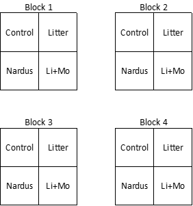
Each block contained four plots, one plot per treatment:
- Control
- Litter – litter was removed
- Nardus – the dominant species, Nardus stricta, was removed
- Li+Mo – litter and moss were removed
In total, there were 16 plots. The experimental design may have looked something like what is shown below, though I suspect the treatments were randomly assigned to the four plots within each block.
Seedlings were identified to species and counted in each plot. In total, 23 species were identified.
The data file, ‘Spackova.et.al.1998.csv’, is available in the GitHub repository. Save this to the ‘data’ subfolder of your class folder. Open the R project for this course, and load the data:
spackova <- read.csv("data/Spackova.et.al.1998.csv", header = T)
The object contains 27 columns: a unique ID code for each plot (plot), the treatment it received (treatment), the block it was in (block), and the total number of seedlings counted (seedlsum), followed by the number of seedlings of each of the 23 species.
Create our imaginary water factor, assigning blocks 1 and 2 to the ‘Yes’ treatment and blocks 3 and 4 to the ‘No’ treatment:
spackova <- spackova %>%

mutate(water = ifelse(block %in% c("Block1", "Block2"), "Yes", "No"))
Verify that this is applied correctly:
unique(spackova[ , c("block", "water")]) block water
1 Block1 Yes
5 Block2 Yes
9 Block3 No
13 Block4 NoBefore we proceed with this analysis, we need to consider how to restrict permutations.
Restricting Permutations in R: the permute package
The vegan package uses several functions to define the order in which permutations are conducted. These functions have been compiled in the permute package, on which vegan depends and which is therefore loaded automatically when vegan is loaded. These functions can be called directly if you want to use them in a permutation test of your own creation (see Simpson 2022 for an example) or from within many of the analytical functions in vegan via the permutations argument. I summarize this approach here; see Simpson (2014, 2022) for details.
The simplest example is one in which all sample units can be freely randomized; in this case, all you need to do is indicate how many permutations you want to conduct. This is done by specifying the number of permutations in the permutations argument, as we’ve done previously. This was also assumed in the shuffle() and shuffleSet() examples above.
More complex designs, such as repeated measures and split-plot designs, require restricted permutations. Several types of permutation are available (Simpson 2022):
- Free permutation (no restrictions)
- Time series or line transect designs – the order of the observations is preserved; permutations simply start at different positions in the series.
- Spatial grid designs – spatial ordering is preserved in both directions
- Permutation of plots or groups of samples
- Blocking factors – groups of sample units that are not permuted themselves, but that permutations are restricted to occur within. An example of this type of design is provided below.
The permute package distinguishes three scales for the purposes of permutations: within, plots, and blocks.
- Blocks are the highest scale. Permutations are restricted so that samples are never permuted among blocks. Blocks must be levels of a factor.
- Plots are the intermediate scale. Samples within a plot can be permuted together, but the plots themselves can also be permuted.
- Within is the lowest scale, and refers to samples nested within plots. If there are no blocks or plots are specified, the permutation instructions specified at this scale are applied to the entire data set.
One limitation of the permute package is that it (at least currently) requires that the dataset be balanced. Unbalanced data would have to be manually permuted.
permute::how()
The how() function is used to specify the details of the permutation design. Its usage is:
how(
within = Within(),
plots = Plots(),
blocks = NULL,
nperm = 199,
complete = FALSE,
maxperm = 9999,
minperm = 5040,
all.perms = NULL,
make = TRUE,
observed = FALSE
)
The main arguments are:
within– permutation design for samples within levels of plots. Produced using another function,Within(), that is described below.plots– permutation design for plots. Produced using another function,Plots(), that is described below.blocks– factor describing the blocking structure. If blocks are present, sample units are permuted within each block but are NOT permuted across blocks.nperm– the number of permutations to perform. Default is 199 but analytical functions may specify a different default number: inadonis2(), the default is 999.complete– whether to conduct all possible permutations. Default is to not do so (FALSE). Note that you would not want to turn this on if the number of permutations is extremely large.minperm– minimum number of permutations at which to conduct all possible permutations. Default is 5040.observed– whether the observed permutation (real data) should be included in the set of all permutations. Default is to not do so (FALSE).
permute::Within() and permute::Plots()
The Within() and Plots() functions have similar usages:
Within(
type = c("free", "series", "grid", "none"),
constant = FALSE,
mirror = FALSE,
ncol = NULL,
nrow = NULL
)
Plots(
strata = NULL,
type = c("none", "free", "series", "grid"),
mirror = FALSE,
ncol = NULL,
nrow = NULL
)
The key arguments are:
strata– a factor; observations from each level are permuted together. Only applies toPlots().type– the key argument in both functions; specifies the type of permutation to be conducted. Four options are possible:free– samples are freely permutedseries– used when the ordering of samples needs to be maintained in one dimension. Intended for temporal data or for spatial data such as that collected along a transect. Adjustments occur by choosing the starting sample, and then maintaining the order of samples that follow. For example, if the numbers (1, 2, 3) are in temporal order, the two possible permutations that maintain this ordering are (2, 3, 1) and (3, 1, 2).grid– used when the ordering of samples needs to be maintained in two spatial dimensions.none– no permutations to be conducted.
constant– whether to use the same permutation within each level ofstrata. Only applies toWithin().
Creating a Permutation Object
The how() and associated functions can be called from within functions such as adonis2(), but this can be confusing and would mean that you have to repeat this information each time you ran the analysis. A more efficient approach is to create a new object containing the permutation instructions and then to call that object as needed. For example:
CTRL <- how(within = Within(type = "free"),
plots = Plots(type = "none"),
nperm = 9999,
observed = TRUE)
In this object, I:
- Specified free permutations of sample units in
within, - Increased the number of permutations from the default (199) to 9999, and
- Included the observed data as one of the permutations when calculating the P-value.
By including all of the key arguments, even if they haven’t been changed, this format is transparent – it is easy to see where changes should be made as appropriate for a given analysis. The blocks argument is absent here but is null unless we specify the factor that we want to use to restrict permutations.
One strong advantage of this approach is that it is easy to apply the same permutation regime to multiple analyses. To use this object, I simply specify ‘permutations = CTRL’ in the arguments for the desired function. For example, we could call the same permutation object when doing a PERMANOVA and a PERMDISP of the same dataset.
Another advantage of this approach is that it is easy to change elements such as the number of permutations. If we change nperm in CTRL, the new number of permutations will automatically be applied to all subsequent analyses using CTRL. By using this permutation object, we don’t have to manually change the number of permutations in each analysis.
Using a Permutation Object
The check() function calculates how many permutations are possible for a given dataset and permutation object. With free permutations, there are a large number of ways to permute the 16 observations in spackova:
check(spackova, control = CTRL)
2.092279e+13However, this ignores the experimental design. For example, the whole plot scale of this design includes four blocks and the (imaginary) water factor. What are the experimental units? Although it is tempting to think about each of the 16 plots as a separate experimental unit, if the entire block was watered at once then the blocks are the experimental units with respect to that factor. Therefore, there are only four experimental units: two watered, two not watered.
During permutations, we recognize that the blocks are the experimental units by keeping the plots within each block together. Another way to say this is that we restrict the permutations to blocks, and do not permute the plots within blocks. We will create a control object (CTRL.b) that does this:
CTRL.b <- how(within = Within(type = "none"),
plots = Plots(strata = spackova$block, type = "free"),
nperm = 999,

observed = TRUE)
Compare the order of the explanatory variables in the original data and in a permutation of the data:
spackova[ , c("plot", "block", "treatment", "water")]
    plot  block treatment water
1   rel1 Block1      Cont   Yes
2   rel2 Block1    Litter   Yes
3   rel3 Block1    Nardus   Yes
4   rel4 Block1     Li+Mo   Yes
5   rel5 Block2      Cont   Yes
6   rel6 Block2    Litter   Yes
7   rel7 Block2    Nardus   Yes
8   rel8 Block2     Li+Mo   Yes
9   rel9 Block3      Cont    No
10 rel10 Block3    Litter    No
11 rel11 Block3    Nardus    No
12 rel12 Block3     Li+Mo    No
13 rel13 Block4      Cont    No
14 rel14 Block4    Litter    No
15 rel15 Block4    Nardus    No
16 rel16 Block4     Li+Mo    No
spackova[shuffle(nrow(spackova), control = CTRL.b) ,
c("plot", "block", "treatment", "water")]
    plot  block treatment water
1   rel1 Block1      Cont   Yes
2   rel2 Block1    Litter   Yes
3   rel3 Block1    Nardus   Yes
4   rel4 Block1     Li+Mo   Yes
13 rel13 Block4      Cont    No
14 rel14 Block4    Litter    No
15 rel15 Block4    Nardus    No
16 rel16 Block4     Li+Mo    No
9   rel9 Block3      Cont    No
10 rel10 Block3    Litter    No
11 rel11 Block3    Nardus    No
12 rel12 Block3     Li+Mo    No
5   rel5 Block2      Cont   Yes
6   rel6 Block2    Litter   Yes
7   rel7 Block2    Nardus   Yes
8   rel8 Block2     Li+Mo   Yes
Verify that the four plots within each block have been permuted as a unit.
Let’s explore the implications of this permutation design:
check(spackova, control = CTRL.b)
24There are only 4 blocks, so there are only 24 possible permutations (i.e., 4!). There are always fewer permutations at the larger scale of a design than at finer scales (e.g., blocks vs. plots in this example), and thus less power to detect effects at the larger scale.
Return to Our Complex (but Realistic) Example
The seedling data are from an experiment testing the effect of four treatments on seedling recruitment. These treatments were applied within blocks. Our (imaginary) watering treatment was applied to blocks. We will analyze each scale separately.
We will also conduct the analysis in a series of steps. To ensure that each step uses the same permutations, we will re-set the random number generator (set.seed()) immediately before each analysis.
Recall that the results of a conventional ANOVA correspond to the results of a PERMANOVA with Euclidean distances. We will use this strategy for verifying the analysis of a complex model as described earlier. We begin by using a simple univariate response, total number of seedlings (seedlsum) to understand the analysis details. Once we have worked through the univariate example, we will apply the correct design to the multivariate response consisting of the germination responses of all 23 species.
Whole Plot Analysis (Water and Block Terms)
The whole plot scale of this design includes the blocks and the (imaginary) water factor. For this portion of the analysis, there are only four experimental units: two watered, two not watered. The treatment term does not relate to variation among blocks so we exclude it from our whole plot model. It will, of course, account for some of the variation within blocks, which we’ll analyze in the split-plot portion of this analysis.
We can use PERMANOVA to test the effects of water and block, applying the CTRL.b permutation object to permute observations within a block as a unit.
set.seed(42)
adonis2(spackova$seedlsum ~ water + block,
data = spackova,

method = "euclidean",
permutations = CTRL.b)
Permutation test for adonis under reduced model
Terms added sequentially (first to last)
Plots: spackova$block, plot permutation: free
Permutation: none
Number of permutations: 24

adonis2(formula = spackova$seedlsum ~ water + block, data = spackova, permutations = CTRL.b, method = "euclidean")
         Df SumOfSqs      R2      F Pr(>F)
water     1    517.6 0.02174 0.2682   0.36
block     2    129.1 0.00542 0.0335   1.00
Residual 12  23159.2 0.97284
Total    15  23805.9 1.00000
I have emphasized the water and block terms in bold.
We arbitrarily assigned the water factor to blocks, so it’s surprising that the water factor accounts for quite a bit of the variation among blocks: SSwater = 517.6 whereas the total variation among blocks is 646.7 (i.e., 517.6 + 129.1).
What is the correct error term for the water factor? There are four blocks so 3 df associated with them. One of these is assigned to the water factor; the other 2 df are associated with other variation among blocks. This is what we need to compare the water factor against. However, the pseudo-F statistic for water that is reported here is incorrect: by back-calculating it using the different terms as its denominator, you can verify that it is based on the residual (i.e., unexplained variation within blocks) rather than the ‘block’ term (i.e., unexplained variation among blocks).
The correct pseudo-F statistic for the water factor in this design would be:
[latex]F = \frac{SS_{water} / df_{water}}{SS_{block} / df_{block}} = \frac{517.6 / 1}{129.1 / 2} = 8.02[/latex]
In the current formulation of adonis2(), we have to calculate this pseudo-F statistic ourselves. Furthermore, if we just calculate if with the real data we don’t have a way to assess its significance. The ‘Step-by-Step Analysis’ section below illustrates how to do this calculation for the real data and for every permutation, so that we can also determine whether it is statistically significant.
The block term accounts for a small amount of variation (SSblock = 129.1); this is the variation among blocks that is not explained by the water factor. Although a pseudo-F statistic and a P-value are reported for the block term, we are not interested in a statistical test of this term and therefore should ignore them. Remember that this is the residual of the whole plot scale.
The variation that is not accounted for by water or block is reported in the Residual (23159.2). All of this variation occurs within blocks, and is therefore the focus of analyses at the split-plot scale. Before we move to that, however, we’ll work through a step-by-step procedure that allows us to calculate the correct pseudo-F statistic for the water factor.
Step-by-Step Analysis (Whole Plot; Manually Calculating pseudo-F-Statistic)
Breaking an analysis into a series of steps can improve our understanding of it. In addition, doing so provides flexibility for situations such as if you wanted to use a term other than the residual as the denominator when calculating a pseudo-F statistic.
In this section, we conduct the whole plot analysis as a series of steps:
- Create a set of permutations
- Apply each permutation to the data, and obtain the SS for each term
- Calculate the pseudo-F-statistic for each permutation
- Use the distribution of F-statistics to determine the P-value for the term of interest
- Summarize the data
1. Create a set of permutations
We begin with the CTRL.b object created above. This object specifies that blocks are to be freely permuted but that plots within blocks are not permuted.
Now, use shuffleSet() to create a set of permutations. The actual ordering of the data is one of the possible permutations, and is the one we are particularly interested in. For simplicity, we will create an object than contains this actual ordering first, followed by multiple random permutations. And, we will re-set the seed of the random number generator first to ensure that we all use the same set of permutations:
set.seed(42)
perms <- rbind(1:nrow(spackova),
shuffleSet(n = nrow(spackova), control = CTRL.b, nset = 999))
#row 1 is the actual data; all others are permutations
The above procedure works well when there are many possible permutations, creating an object in which each row is a permutation (actually, real data + permutations) and each column indexes a sample unit. However, in this case there are only 4 blocks and thus 24 permutations. The shuffleSet() function identified this and generated the set of all possible permutations. This complicates our object a little bit because it contains the actual ordering of the data twice (verify that this is the case). By viewing the perms object, you can verify that the first two rows are identical – in other words, the complete set of permutations begins with the real data. This isn’t the case when we generate a subset of the permutations, which is why we include it in perms. For this particular situation, we’ll drop the second row:
perms <- perms[ -2 , ]
The resulting object contains all possible permutations of the four blocks, keeping the observations within each block together.
head(perms)
     [,1] [,2] [,3] [,4] [,5] [,6] [,7] [,8] [,9] [,10] [,11] [,12] [,13] [,14] [,15] [,16]
[1,]    1    2    3    4    5    6    7    8    9    10    11    12    13    14    15    16
[2,]    1    2    3    4    5    6    7    8   13    14    15    16     9    10    11    12
[3,]    1    2    3    4    9   10   11   12    5     6     7     8    13    14    15    16
[4,]    1    2    3    4    9   10   11   12   13    14    15    16     5     6     7     8
[5,]    1    2    3    4   13   14   15   16    5     6     7     8     9    10    11    12
[6,]    1    2    3    4   13   14   15   16    9    10    11    12     5     6     7     8
2. Apply each permutation to the data and obtain the SS for each term
We will use a for() function to loop through the permutations. For each permutation, we will conduct a PERMANOVA with water and block as terms, and then extract the SS for all terms.
We begin by creating an object where the resulting SS can be stored. We need to anticipate the structure of the analysis to create this results object. In this case, there will be four SS (water, block, residual, total; see the PERMANOVA table above), so we will create a column for each and name them in the order they are reported in the results. We create a row in results for each permutation to be tested.
results <- matrix(nrow = nrow(perms), ncol = 4)
colnames(results) <- c("water", "block", "residual", "total")
Now we loop through the permutations. For each permutation (row from perms), we permute the explanatory factors, conduct a PERMANOVA of the response, and save the SS associated with each term to that row of the results object.
for (i in 1:nrow(perms)) {
temp.data <- spackova[perms[i, ], ]
temp <- adonis2(spackova$seedlsum ~ water + block,
  data = temp.data,

method = "euclidean",

permutations = 0)
results[i, ] <- t(temp$SumOfSqs)
}
A few notes on this loop:
- The data object is indexed using
perms[i,]– this is what shuffles the water and block codes so that they are re-assigned to a new row of data. - The response variable is indexed fully (
spackova$seedlsum) rather than just calling the column (seedlsum). If we did the latter, the response would be found within thedataargument and therefore would have been permuted just like the water and block terms. - The number of permutations within each loop is set to zero as we are manually looping through the permutations and therefore don’t need to do any permutations within each loop.
- The SS from permutation
iare saved to rowiofresults. - This code uses
adonis2(). Other functions could be used instead, but the resulting object would have a different structure and therefore a different type of indexing would be required to extract the SS. - If you want to re-run this loop, you should re-create
resultsobject first. Otherwise, each new iteration of the loop will add its output to the end of the object that already contains data from a previous run of the loop.
Customizing this code for a different analysis would require adjusting the number and names of columns within results and the model formulation within adonis2().
3. Calculate the pseudo-F-statistic for each permutation
View the first few rows from results:
head(results)
        water   block residual    total
[1,] 517.5625 129.125 23159.25 23805.94
[2,] 517.5625 129.125 23159.25 23805.94
[3,]  52.5625 594.125 23159.25 23805.94
[4,]  76.5625 570.125 23159.25 23805.94
[5,]  52.5625 594.125 23159.25 23805.94
[6,]  76.5625 570.125 23159.25 23805.94
The residual SS and total SS are unchanged from one permutation to another. What we have done here has only altered the SS for water and for block.
The test statistic in PERMANOVA is a pseudo-F-statistic, which is calculated just like a classical F-statistic. The error term for water is the block term – the unexplained variation among blocks – so we calculate the pseudo-F-statistic for it as the mean square (MS) for water divided by the mean square for block. We can calculate these for every permutation en masse:
results <- results |>
data.frame() |>
mutate(F.water = (water/1)/(block/2))
This calculation of the test statistic using a term other than the residual as the denominator is something that cannot be controlled in the current formulation of adonis2(). We could have done this calculation within the loop and saved just the values of this test statistic rather than the SS of each term – I did not do so as I want the analysis to be transparent. It is also more efficient to do this calculation once at the end rather than repeat it for each loop.
I hard-coded the df in the calculation of the pseudo-F-statistic. This would have to be customized for other datasets.
The pseudo-F-statistic from the real data is in row 1 because it was the first row in our perms object:
results[1,] # all data from real data
     water   block residual    total  F.water
1 517.5625 129.125 23159.25 23805.94 8.016457
Verify that these SS match those that we calculated above and that this pseudo-F-statistic agrees with what we expected when we calculated it manually.
4. Use the distribution of F-statistics to determine the P-value for the term of interest
The P-value for the water term is the proportion of permutations with a pseudo-F-statistic as large or larger than that calculated from the real data:
with(results, sum(F.water >= F.water[1]) / length(F.water))
0.125In this case, there are few permutations (24) and even fewer unique combinations (6), and therefore it is mathematically impossible for the p-value to be statistically significant. We could graph the distribution of F-statistics as we’ve done in other notes, but in this case the low number of permutations makes it pretty boring (give it a try!).
5. Summarize the results
In this analysis, F = 8.02 and P = 0.125. We conclude that our imaginary water factor has no effect on total seedling recruitment.
Split Plot Analysis (Treatment Term)
Analyses at the split-plot scale focus on terms that vary within the whole plots. However, this doesn’t mean that we can ignore the whole plots – if we omit them from our model, the variation they explain will be added to the residual. Furthermore, this is an example of how the design of an experiment should dictate the structure of the analysis.
Although we need to account for the variation among blocks, in this analysis we are not interested in statistical tests of this variation. Therefore we can let the block term represent all variation among blocks. In other words, we don’t need to partition the variation due to our imaginary water factor from that which cannot be explained by that factor.
We generally include a blocking term as the first term in a split plot model. This technically doesn’t matter if our data are balanced, but is helpful in case the data are unbalanced as it ensures that the blocking term accounts for as much variation as possible when using Type I SS (review the notes on this topic if this seems unfamiliar).
In addition to including the blocking term so that the variation is partitioned correctly, we also need to account for it when permuting the treatments. It may be helpful to view the schematic of the experimental design to demonstrate why this restriction is necessary. If we allowed permutations to occur freely among all plots, permutations could ‘mix’ the variation among treatments within the same block with the variation among plots from different blocks – and the latter variation is not due to treatment alone. Since our intent is to focus on the variation among treatments, we need to restrict the permutations so that plots are permuted within each block, but plots are not permuted across blocks.
Here are two ways to permute the treatment factor without permuting the block factor:
CTRL.t <- how(within = Within(type = "free"),
plots = Plots(type = "none"),

blocks = spackova$block,
nperm = 999,

observed = TRUE)
CTRL.t <- how(within = Within(type = "free"),
plots = Plots(strata = spackova$block, type = "none"),
nperm = 999,

observed = TRUE)
The terminology here is a bit confusing, as we are assigning blocks to the plots argument. Refer back to the notes about restricting permutations above for an explanation of the arguments within the how() function.
These objects are functionally equivalent – they specify that plots are to be freely permuted within blocks but that blocks are not allowed to permute.
There are a much larger number of permutations for this permutation object than for CTRL.b above:
check(spackova, control = CTRL.t)
331776Earlier we viewed the original explanatory information and how it was altered by the CTRL.b object. We can do the same with this permutation object:
spackova[shuffle(nrow(spackova), control = CTRL.t) ,
c("plot", "block", "treatment", "water")]
    plot  block treatment water
1   rel1 Block1      Cont   Yes
4   rel4 Block1     Li+Mo   Yes
3   rel3 Block1    Nardus   Yes
2   rel2 Block1    Litter   Yes
6   rel6 Block2    Litter   Yes
8   rel8 Block2     Li+Mo   Yes
7   rel7 Block2    Nardus   Yes
5   rel5 Block2      Cont   Yes
12 rel12 Block3     Li+Mo    No
11 rel11 Block3    Nardus    No
10 rel10 Block3    Litter    No
9   rel9 Block3      Cont    No
16 rel16 Block4     Li+Mo    No
13 rel13 Block4      Cont    No
15 rel15 Block4    Nardus    No
14 rel14 Block4    Litter    No
Verify that treatments are being permuted within blocks but that the blocks themselves have not changed.
Now, we apply the CTRL.t object within our analysis:
set.seed(42)
adonis2(spackova$seedlsum ~ block + treatment,
data = spackova,

method = "euclidean",
permutations = CTRL.t)
Permutation test for adonis under reduced model
Terms added sequentially (first to last)
Plots: spackova$block, plot permutation: none
Permutation: free
Number of permutations: 999

adonis2(formula = spackova$seedlsum ~ block + treatment, data = spackova, permutations = CTRL.t, method = "euclidean")
          Df SumOfSqs      R2      F Pr(>F)
block      3    646.7 0.02716 0.2017  0.051 .
treatment  3  13539.7 0.56875 4.2225  0.051 .
Residual   9   9619.6 0.40408
Total     15  23805.9 1.00000
---
Signif. codes:  0 ‘***’ 0.001 ‘**’ 0.01 ‘*’ 0.05 ‘.’ 0.1 ‘ ’ 1
Block is added first to ensure that it accounts for as much of the variation as possible. There are 3 df for block, and this accounts for all of the variation partitioned to the water and block terms in the whole plot analysis. Since the blocks were not permuted, the P-value for this term should be ignored (see above section about testing this term). Gavin Simpson, the author and maintainer of the permute package, is uncertain why the P-value from the treatment term is also reported for the block term.
The variation that was unexplained in the whole plot analysis (Residual SS of 23159.3 in that analysis) has now been partitioned into that which can be explained by treatment (SStreatment = 13539.7) and that which cannot (SSResidual = 9619.6). The treatment term is highlighted in bold. It accounts for more than half of the variation in seedling recruitment (partial R2 = 0.57).
The pseudo-F-statistic for the treatment term has been correctly calculated using the residual in its denominator. This term is marginally significant. We can get a more precise estimate of the significance of treatment by increasing the number of permutations – let’s do 100,000 permutations now:
CTRL.t <- how(within = Within(type = "free"),
plots = Plots(type = "none"),
blocks = spackova$block,
nperm = 99999,
observed = TRUE)
set.seed(42)
adonis2(spackova$seedlsum ~ block + treatment,
data = spackova,
method = "euclidean",
permutations = CTRL.t)
Permutation test for adonis under reduced model
Terms added sequentially (first to last)
Blocks:  spackova$block
Permutation: free
Number of permutations: 99999

adonis2(formula = spackova$seedlsum ~ block + treatment, data = spackova, permutations = CTRL.t, method = "euclidean")
          Df SumOfSqs      R2      F  Pr(>F)
block      3    646.7 0.02716 0.2017 0.04634 *
treatment  3  13539.7 0.56875 4.2225 0.04634 *
Residual   9   9619.6 0.40408
Total     15  23805.9 1.00000
---
Signif. codes:  0 ‘***’ 0.001 ‘**’ 0.01 ‘*’ 0.05 ‘.’ 0.1 ‘ ’ 1
It appears that treatment has a weakly significant effect on overall seedling recruitment.
Summary: Whole and Split Plot Analyses Together
Once we have analyzed each term correctly, we can build a summary ANOVA table which shows how the variance was partitioned for each term. Here, I combine the details of the correct analyses from above.
| df | SS | pseudo-F | P | |
| Whole Plot | ||||
| water | 1 | 517.6 | 8.02 | 0.125 |
| block | 2 | 129.1 | ||
| Split Plot | ||||
| treatment | 3 | 13539.7 | 4.22 | 0.046 |
| Residual | 9 | 9619.6 | ||
| Total | 15 | 23805.9 |
In the whole plot analysis portion of this table, the pseudo-F-statistic and P-value for the water factor are those that we calculated in the step-by-step procedure above. A pseudo-F-statistic and P-value are not reported for block because we are not testing that term statistically.
In the split-plot analysis portion of this table, we focus just to treatment and the unexplained variation among plots; the block term has already been reported in the whole plot analysis table. We conclude that total seedling germination differs marginally among treatments. If interested, we could use pairwise comparisons to determine which treatments it differs amongst.
Comparison with ANOVA
For comparison, here is a univariate ANOVA of the same data. The Error() within the formula is how the aov() function specifies that a term other than the residual should be used as an error term.
summary(aov(spackova$seedlsum ~ water + Error(block) + treatment,

data = spackova))
Error: block
          Df Sum Sq Mean Sq F value Pr(>F)
water      1  517.6   517.6   8.016  0.105
Residuals  2  129.1    64.6

Error: Within
          Df Sum Sq Mean Sq F value Pr(>F)
treatment  3  13540    4513   4.223 0.0403 *
Residuals  9   9620    1069
---
Signif. codes:  0 ‘***’ 0.001 ‘**’ 0.01 ‘*’ 0.05 ‘.’ 0.1 ‘ ’ 1
You can verify that this ANOVA table is identical to what we calculated via PERMANOVA above, except for the P-values. There are also a few rounding and formatting differences – for example, I included a row for the total, while the ANOVA table contains the mean square values – but these differences do not alter the interpretation.
Incorrect Analyses
There are many ways to analyze data incorrectly. For example, we could:
- Analyze the entire dataset as a completely random design (no restrictions on permutations, use of residual in error term of all test statistics)
- Ignore the block term while analyzing the effect of treatment
- Restrict permutations incorrectly
The omission of necessary factors or inclusion of unnecessary factors can alter how the variation is partitioned. As discussed above, when a term is omitted, the variation that is associated with it, and the associated df, are assigned to the residual. How much this alters the conclusions will depend greatly on how much variance the omitted term explains. For example, if a term would have explained a lot of variation in the data, then its omission would greatly increase the residual SS and thus would reduce the F-statistic for other terms that used the residual as the denominator in its calculation. If a term was associated with lots of df (e.g., a factor with multiple levels), then its omission will increase the df of the residual and therefore can reduce the residual MS and increase the F-statistic for other terms that use the residual as the denominator.
Restricting the permutations incorrectly can alter the statistical significance associated with a given value of a test statistic. This could happen if we don’t have the permutation object specified correctly or if we call the wrong one (e.g., apply CTRL.b in the split plot analysis, or apply CTRL.t in the whole plot analysis).
Bottom line: think through the analysis process carefully, and to document your decisions in a script.
Analysis of A Multivariate Response
Switching from a univariate PERMANOVA to a multivariate PERMANOVA is trivial – we simply change the response specified in the model to the desired multivariate response, with the desired distance measure. Here, we’ll focus on composition, expressing the number of seedlings of each species as a proportion of the plot total.
Create Response Object
To begin, we extract the data and standardize by plot totals.
spackova.comp <- spackova |>
select(-c(plot, treatment, block, seedlsum, water)) |>
decostand(method = "total")
This is our new response object.
Conduct Whole Plot Analysis
We use the same approach as above, restricting permutations so that blocks are permuted while plots within blocks are permuted together. Since we need to manually calculate the F-statistic for the water term, we’ll use the step-by-step procedure shown above.
Note: I had to update the name of the response object within the for() loop below – this is shown in red font. This is the only element of the code that needed to be changed from what we used in the univariate analysis.
set.seed(42)
perms <- rbind(1:nrow(spackova),
shuffleSet(n = nrow(spackova), control = CTRL.b, nset = 999))

#
row 1 is the actual data; all others are permutations
perms <- perms[ -2 , ] #remove duplicated actual data order
results <- matrix(nrow = nrow(perms), ncol = 4)
colnames(results) <- c("water", "block", "residual", "total")
for (i in 1:nrow(perms)) {
temp.data <- spackova[perms[i, ], ]
temp <- adonis2(spackova.comp ~ water + block,
  data = temp.data,

method = "euclidean",

permutations = 0)
results[i, ] <- t(temp$SumOfSqs)
}
results <- results %>%

data.frame() %>%

mutate(F.water = (water/1)/(block/2))
Now we can extract the pseudo-F-statistic from the actual data:
results[1,] # all data from real data
      water     block  residual    total  F.water
1 0.1071991 0.1626741 0.9706154 1.240489 1.317961
Calculate the P-value:
with(results, sum(F.water >= F.water[1]) / length(F.water))
0.6666667Conduct Split-plot Analysis
set.seed(42)
adonis2(spackova.comp ~ block + treatment,

data = spackova,

method = "euclidean",

permutations = CTRL.t)
Permutation test for adonis under reduced model
Terms added sequentially (first to last)
Blocks:  spackova$block
Permutation: free
Number of permutations: 99999

adonis2(formula = spackova.comp ~ block + treatment, data = spackova, permutations = CTRL.t, method = "euclidean")
          Df SumOfSqs      R2      F Pr(>F)
block      3  0.26987 0.21755 1.0891 0.5549
treatment  3  0.22724 0.18318 0.9170 0.5549
Residual   9  0.74338 0.59926
Total     15  1.24049 1.00000
Although we included both terms in this model, we focus our attention only on the treatment term.
Summarize Results
Finally, we summarize these results in an ANOVA table:
| df | SS | pseudo-F | P | |
| Whole Plot | ||||
| water | 1 | 0.107 | 1.32 | 0.667 |
| block | 2 | 0.163 | ||
| Split Plot | ||||
| treatment | 3 | 0.227 | 0.92 | 0.555 |
| Residual | 9 | 0.743 | ||
| Total | 15 | 1.240 |
In this case, there is no evidence of a compositional difference due to either our imaginary water factor (it would be strange if it was significant!) or among treatments. Given our earlier analysis of total seedling numbers, this implies that the treatments affected overall recruitment but do not favor particular species.
It is ecologically possible that the treatments favor particular species at particular blocks. Statistically, this would be tested by examining a block x treatment interaction. However, this interaction can only be tested if there are replicate plots within blocks. Without that replication, as in this example, the block x treatment interaction functions as the whole plot error term (residual).
Conclusions
The variance is partitioned by including the correct terms in the model and ensuring that the correct term is used as the error term (denominator) when calculating the test statistic.
The P-value is determined by restricting permutations appropriately.
How much of a difference these decisions make on your conclusions will depend on the characteristics of the data being analyzed and the terms across which the restrictions occur.
One caveat to keep in mind: the permute() function is designed for balanced data. If your data are unbalanced (e.g., different numbers of subsamples in each sample unit), you would have to develop the permutations more carefully. This could be done in several ways, including:
- Permute sample unit IDs and then manually assign those permutation sequences to all subsamples within each sample unit.
- Drop data to create a balanced design. Depending on the dataset, data to drop could be selected randomly, by excluding one level of a treatment if that level is missing observations, etc.
- Conduct a Principal Coordinates Analysis (PCoA), retaining all axes, and then calculate the centroid for each sample unit. An advantage of this approach is that it can be applied to any distance measure. For scale-dependent variables such as composition, it would not be appropriate to compare averages if those averages were based on different numbers of subsamples. We’ll illustrate this idea when we talk about PCoA.
References
Anderson, M.J., and C.J.F. ter Braak. 2003. Permutation tests for multi-factorial analysis of variance. Journal of Statistical Computation and Simulation 73:85-113.
Green, R.H. 1993. Application of repeated measures designs in environmental impact and monitoring studies. Australian Journal of Ecology 18:81-98.
Hurlbert, S.H. 1984. Pseudoreplication and the design of ecological field experiments. Ecological Monographs 54:187-211.
Mitchell et al. 2017. Power? Wainwright?
Simpson, G.L. 2014. Analysing a randomized complete block design with vegan. http://www.fromthebottomoftheheap.net/2014/11/03/randomized-complete-block-designs-and-vegan/
Simpson, G.L. 2022. Restricted permutations; using the permute package. https://cran.r-project.org/web/packages/permute/vignettes/permutations.html
Šmilauer, P., and J. Lepš. 2014. Multivariate Analysis of Ecological Data Using CANOCO 5. 2 edition. Cambridge University Press.
Somerfield, P.J., K.R. Clarke, and R.N. Gorley. 2021a. A generalized analysis of similarities (ANOSIM) statistic for designs with ordered factors. Austral Ecology 46:901-910.
Somerfield, P.J., K.R. Clarke, and R.N. Gorley. 2021b. Analysis of similarities (ANOSIM) for 2-way layouts using a generalized ANOSIM statistic, with comparative notes on Permutational Multivariate Analysis of Variance (PERMANOVA). Austral Ecology 46:911-926.
Somerfield, P.J., K.R. Clarke, and R.N. Gorley. 2021c. Analysis of similarities (ANOSIM) for 3-way designs. Austral Ecology 46:927-941.
Špačková, I., I. Kotorová, and J. Lepš. 1998. Sensitivity of seedling recruitment to moss, litter and dominant removal in an oligotrophic wet meadow. Folia Geobotanica 33:17–30. http://doi.org/10.1007/BF02914928
Media Attributions
- analysis.flowchart
- Spackova
