Introduction

k-means cluster analysis is a non-hierarchical technique.  It seeks to partition the sample units into k groups in a way that minimizes some criterion. Often, the criterion relates to the variance between points and the centroid of the groups they are assigned to.

An essential part of a k-means cluster analysis, of course, is the decision of how many clusters to include in the solution.  One way to approach this is to conduct multiple analyses for different values of k and to then compare those analyses.  For example, Everitt & Hothorn (2006) provide some nice code to compare the within-group sums of squares against k.  Another approach is to use the results of a hierarchical clustering method as the starting values for a k-means analysis.  One of the older posts on Stack Overflow contains many examples of how to determine an appropriate number of clusters to use in a k-means cluster analysis.  Additional ideas about how to decide how many clusters to use are provided below.

The criterion in k-means clustering is generally to minimize the variance within groups, but how variance is calculated varies among algorithms.  For example, kmeans() seeks to minimize within-group sums of squared distances. Another function, pam(), seeks to minimize within-group sums of dissimilarities, and can be applied to any distance matrix.  Both functions are described below.

k-means cluster analysis is an iterative process:

• Select k starting locations (centroids)
• Assign each observation to the group to which it is closest
• Calculate within-group sums of squares (or other criterion)
• Adjust coordinates of the k locations to reduce variance
• Re-assign observations to groups, re-assess variance
• Repeat process until stopping criterion is met

The iterative nature of this technique can be seen using the animation::kmeans.ani() function (see the examples in the help files) or in videos like this: https://www.youtube.com/watch?v=BVFG7fd1H30.  We will see a similar iterative process with NMDS.

k-means clustering may find a local (rather than global) minimum value due to differences in starting locations.  A common solution to this is to use multiple starts, thus increasing the likelihood of detecting a global minimum.  This, again, is similar to the approach taken in NMDS.

As usual, we will illustrate these approaches with our oak dataset.

source("scripts/load.oak.data.R")

k-means Clustering in R

In R, k-means cluster analysis can be conducted using a variety of methods, including stats::kmeans(), cluster::pam(), cluster::clara(), and cluster::fanny().

stats::kmeans()

The kmeans() function is available in the stats package.  It seeks to identify the solution that minimizes the sum of squared (Euclidean) distances.  Its usage is:

kmeans(x,
centers,
iter.max = 10,
nstart = 1,
algorithm = c("Hartigan-Wong", "Lloyd", "Forgy", "MacQueen"),
trace = FALSE
)

The key arguments are:

• x – data matrix.  Note that a distance matrix is not allowed.  Euclidean distances are assumed to be appropriate.
• centers – the number of clusters to be used.  This is the ‘k’ in k-means.
• iter.max – maximum number of iterations allowed.  Default is 10.
• nstart – number of random sets of centers to choose.  Default is 1.
• algorithm – the algorithm used to derive the solution.  I won’t pretend to understand what these algorithms are or how they differ.  🙂  The default is “Hartigan-Wong“.

This function returns an object of class ‘kmeans’ with the following values:

• cluster – a vector indicating which cluster each sample unit is assigned to.  Note that the coding of clusters is arbitrary, and that different runs of the function may result in different coding.
• centers – a matrix showing the mean value of each species in each sample unit.
• totss – the total sum of squares.
• withinss – the within-cluster sum of squares for each cluster.
• tot.withinss – the sum of the within-cluster sum of squares
• betweenss – the between-cluster sum of squares.
• size – the number of sample units in each cluster.
• iter – the number of iterations

An example for six groups:

k6 <- kmeans(x = Oak1, centers = 6, nstart = 100)

Note that we did not make any adjustments to our data but are using this here to illustrate the technique.  Also, your results may differ depending on the number of starts (nstart) and the number of iterations (iter.max).  In addition, your groups may be identified by different integers.  To see the group assignment of each sample unit:

k6$cluster

Stand01 Stand02 Stand03 Stand04 Stand05 Stand06 Stand07 
      1       1       1       5       4       2       1 
Stand08 Stand09 Stand10 Stand11 Stand12 Stand13 Stand14 
      5       5       6       1       1       1       1 
Stand15 Stand16 Stand17 Stand18 Stand19 Stand20 Stand21 
      4       6       5       5       4       1       1 
Stand22 Stand23 Stand24 Stand25 Stand26 Stand27 Stand28 
      5       3       5       1       4       1       4 
Stand29 Stand30 Stand31 Stand32 Stand33 Stand34 Stand35 
      4       5       4       4       2       5       1 
Stand36 Stand37 Stand38 Stand39 Stand40 Stand41 Stand42 
      3       4       4       1       4       2       4 
Stand43 Stand44 Stand45 Stand46 Stand47 
      2       6       5       5       5 

A more compact summary:

table(k6$cluster)

 1  2  3  4  5  6 
 2 12 12 14  3  4

vegan::cascadeKM()

The kmeans() function permits a cluster analysis for one value of k.  The cascadeKM() function, available in the vegan package, conducts multiple kmeans() analyses: one for each value of k ranging from the smallest number of groups (inf.gr) to the largest number of groups (sup.gr):

cascadeKM(Oak1, inf.gr = 2, sup.gr = 8)

(output not displayed in notes)

The output can also be plotted:

plot(cascadeKM(Oak1, inf.gr = 2, sup.gr = 8))

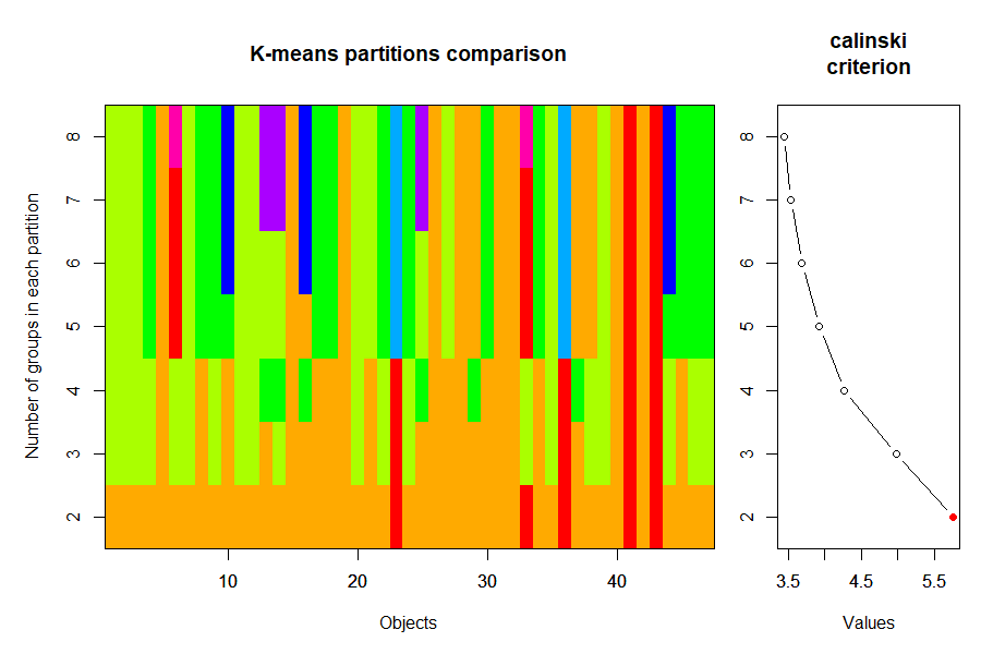
It is important to recall that k-means solutions are not hierarchical – you can see evidence of this by looking at the colors in this graph.

cluster::pam()

The pam() function is available in the cluster package.  The name is an abbreviation for ‘partitioning around medoids’ (a medoid is a representative example of a group – in this case, the sample unit that is most similar to all other sample units in the cluster).  It is more flexible than kmeans() because it allows the use of distance matrices produced from non-Euclidean measures.  It also uses a different criterion, identifying the solution that minimizes the sum of dissimilarities.  Its usage is:

pam(x,
k,
diss = inherits(x, "dist"),
metric = c("euclidean", "manhattan"),
medoids = if (is.numeric(nstart)) "random",
nstart = if (variant == "faster") 1 else NA,
stand = FALSE,
cluster.only = FALSE,
do.swap = TRUE,
keep.diss = !diss && !cluster.only && n < 100,
keep.data = !diss && !cluster.only,
variant = c("original", "o_1", "o_2", "f_3", "f_4", "f_5", "faster"),
pamonce = FALSE,
trace.lev = 0
) 

There are quite a few arguments in this function, but the key ones are:

• x – data matrix or data frame, or distance matrix.  Since this accepts a distance matrix as an input, it does not assume Euclidean distances as is the case with kmeans().
• k – the number of clusters to be used
• diss – logical; x is treated as a distance matrix if TRUE (default) and as a data matrix if FALSE.
• metric – name of distance measure to apply to data matrix or data frame.  Options are “euclidean” and “manhattan“.  Ignored if x is a distance matrix.
• medoids – if you want specific sample units to be the medoids, you can specify them with this argument.  The default (NULL) results in the medoids being identified by the algorithm.
• stand – whether to normalize the data (i.e., subtract mean and divide by SD for each column). Default is to not do so (FALSE).  Ignored if x is a dissimilarity matrix.

This function returns an object of class ‘pam’ that includes the following values:

• medoids – the identity of the sample units identified as ‘representative’ for each cluster.
• clustering – a vector indicating which cluster each sample unit is assigned to.
• silinfo – silhouette width information.  The silhouette width of an observation compares the average dissimilarity between it and the other points in the cluster to which it is assigned and between it and points in other clusters.  A larger value indicates stronger separation or strong agreement with the cluster assignment.

An example for six groups:

k6.pam <- pam(x = Oak1.dist, k = 6)

Note that we called Oak1.dist, which is based on Bray-Curtis dissimilarities, directly since pam() cannot calculate this measure internally.  Your groups may be identified by different integers.  To see the group assignment of each sample unit:

k6.pam$clustering

Stand01 Stand02 Stand03 Stand04 Stand05 Stand06 Stand07 
      1       1       1       2       3       1       1 
Stand08 Stand09 Stand10 Stand11 Stand12 Stand13 Stand14 
      2       2       4       2       1       5       5 
Stand15 Stand16 Stand17 Stand18 Stand19 Stand20 Stand21 
      4       5       3       3       3       2       3 
Stand22 Stand23 Stand24 Stand25 Stand26 Stand27 Stand28 
      2       6       2       5       4       3       4 
Stand29 Stand30 Stand31 Stand32 Stand33 Stand34 Stand35 
      5       4       4       3       6       3       2 
Stand36 Stand37 Stand38 Stand39 Stand40 Stand41 Stand42 
      6       4       2       4       4       6       2 
Stand43 Stand44 Stand45 Stand46 Stand47 
      6       2       2       2       2

The integers associated with each stand indicate the group to which it is assigned.

The help file about the object that is produced by this analysis (?pam.object) includes an example in which different numbers of clusters are tested systematically and the size with the smallest average silhouette width is selected as the best number of clusters.  Here, I’ve modified this code for our oak plant community dataset:

asw <- numeric(10)
for (k in 2:10) {
  asw[k] <- pam(Oak1.dist, k = k) $ silinfo $ avg.width
}
cat("silhouette-optimal # of clusters:", which.max(asw), "\n")

silhouette-optimal # of clusters: 2 

This algorithm suggests that there is most support for two clusters of sample units.  We could re-run pam() with this specific number of clusters if desired.

Comparing k-means Analyses

Many of the techniques that we saw previously for comparing hierarchical cluster analyses are also relevant here.  For example, we could generate a confusion matrix comparing the classifications from the kmeans() and pam().

table(k6$cluster, k6.pam$clustering)

    1 2 3 4 5 6
  1 5 3 2 1 3 0
  2 1 0 0 0 0 3
  3 0 8 3 1 0 0
  4 0 0 0 0 0 2
  5 0 1 0 1 1 0
  6 0 2 3 6 1 0

This can be a bit confusing to read because the row and column names are the integers 1:6 but the cells within the table are also numbers (i.e., number of stands in each group).   Also, the number of groups is the same in both analyses so it isn’t immediately apparent which analysis is shown as rows and which as columns.

Note that observations are more easily assigned to different groups in k-means analyses than they are in hierarchical analysis: in the latter, once two sample units are fused together they remain fused through the rest of the analysis.

Conclusions

k-means cluster analysis is a technique for classifying sample units into k groups.  This approach is not constrained by the decisions that might have been made earlier in a hierarchical analysis.  There is also no concern about other factors such as which group linkage method to use.

However, k-means cluster analysis does require that the user decide how many groups (k) to focus on.  In addition, since the process is iterative and starts from random coordinates, it’s possible to end up with different classifications from one run to another.  Finally, functions such as kmeans() use a Euclidean criterion and thus are most appropriate for data expressed with that distance measure.  To apply this technique to a semimetric measure such as Bray-Curtis dissimilarity, some authors have suggested standardizing data using a Hellinger transformation: the square root of the data divided by the row total.  This standardization is available in decostand(), but I have not explored its utility.

References

Everitt, B.S., and T. Hothorn. 2006. A handbook of statistical analyses using R. Chapman & Hall/CRC, Boca Raton, LA.