
Foundational Concepts
1 Installing and Running Software
Learning Objectives
To demonstrate how to install R and RStudio software.
To become familiar with ways of navigating in R.
To learn how to install, load, and update R packages.
To understand how R help files are structured.
Resources
RStudio cheat sheets for reference:
Introduction
Installing and Running R
The official R website is: http://cran.r-project.org/. However, there are multiple mirrors that contain the exact same information. You can choose the mirror that is nearest your location. Go to the R website (or a mirror), and choose the appropriate operating system from the top center of the page (box titled ‘Download and Install R’).
- Windows: Click on ‘base’, and then on the setup program (currently R-4.3.2-win.exe). Save this file to a working directory.
- Mac: Choose the setup program. Save this file to a working directory.
Once the file has downloaded, double-click on it to run it. Accept all defaults to install it on your hard drive.
If you would like to install R on a thumb drive (with enough room!), change the install destination during the installation, and choose NOT to create a Start Menu folder or desktop icon. Accept all other defaults. (Note: I haven’t fully tested this; you may need to install software to create a virtual PC on your thumb drive first). For more details, see Appendix A of Dalgaard (2008) or Torfs & Brauer (2014).
By default, R operates from a command line interface. When you open R, the main window is displayed. This window, called the ‘R Console’, is where commands are executed, and their numerical/textual results displayed.
R also uses several other windows:
- Graphics
- Editor
- Data editor
These windows are only displayed when necessary. The Editor window is where multiple lines of commands can be written and saved. This permits you to execute a series of commands sequentially. It is extremely useful for saving code so it can easily be rerun in the future.
Installing and Running RStudio
While the standard installation of R does not include a graphical user interface (GUI), several are available as packages that can be installed. In this course, we will not be using a GUI as I want you to see and understand what is happening throughout the analyses. However, the default setting of R is not entirely satisfactory either. Instead, we will use RStudio, an IDE (‘integrated development environment’) for R that is available as a free download.
RStudio is available from https://posit.co/download/rstudio-desktop/. The current version is 2023.09.1+494.
A guide to RStudio is provided on the RStudio IDE cheat sheet. More detail is available in the book by van der Loo & de Jonge (2012).
When you open RStudio, R is automatically opened as well. The version that is running is displayed in the Console. If you have multiple versions of R installed, you can select the version that you want to use. To do so, go to ‘Tools / Global Options’ and select the ‘Change…’ button below R Version. A list of the installed versions will be displayed; select the one you desire. You may have to restart RStudio for this to take effect.
RStudio Basics
The RStudio window is divided into several panes as shown and described below.
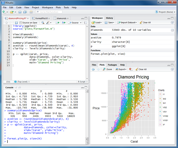
In the lower left is the R Console – the same as you see when you open R directly. There are also tabs here for Terminal and Background Jobs.
In the upper left is an editor pane (this may not be displayed if you have not opened or created a script). The editor pane is where you can open, edit, and save a script file containing many lines of code. This is analogous to the editor window in R, but has additional features such as:
- Multiple scripts can be open simultaneously, each appearing as a tab in this pane.
- Font color changes to distinguish functions, comments, etc.
- Auto-complete: when you type a left parenthesis or bracket, the closing parenthesis or bracket is automatically created.
- Quotation marks: if you need to place material in quotation marks, you can do so by highlighting it and then typing the quotation mark – they are automatically added before and after the selected text.
- Error-checking: when you place the cursor after a parenthesis, the corresponding parenthesis that closes the clause is highlighted. This is particularly helpful when you have multiple functions nested one inside another.
- Can comment or uncomment multiple lines simultaneously (Edit tab: Comment/Uncomment Lines’ command).
In the upper right pane are four tabs:
- Environment: displays summary details of the objects you have created in R (more on those later).
- History: a list of all of the commands that you’ve run during this session, in order.
- Connections: allows you to connect to different data sources.
- Tutorial: allows you to run tutorials about RStudio.
Finally, the lower right pane contains six tabs:
- Files: allows simple navigation within your directory structure.
- Plots: displays the graphics that you produce through commands sent to the Console. Can move left to right to move between figures.
- Packages: allows you to load or remove packages by simply selecting the checkbox beside their name. Packages that are not installed (see below) are not included in this list.
- Help: access to the help files associated with the base version of R and with installed packages.
- Viewer: to view local web content.
- Presentation: ability to create and display presentations that include R code and output.
Navigating in R
The ‘>’ prompt in the R Console indicates that R is waiting for a command.
You can execute commands from RStudio’s editor pane by clicking ‘Run’ or pressing the Ctrl-Enter key combination. Selecting code before executing will alter what is run:
- Place the cursor anywhere in a line of code (note: does not have to be at the end of the line). ‘Run’ will execute that line of code. If the line is part of a set of commands, the full set will be run. However, this is not true if the commands are embedded within other types of instructions. For example, a function consists of code ‘wrapped’ by commands about argument names, etc. Placing the cursor in a line of code within a function will run the code but not the associated wrapper lines.
- Highlight multiple lines of code. ‘Run’ will execute all of the highlighted code.
- Highlight a portion of a line. ‘Run’ will execute just the highlighted text and not the rest of the line. This can be helpful when debugging code, for example as it allows you to execute one portion at a time.
Once you’ve entered a command, you can use the up arrow to scroll through commands you’ve already run. You can then edit and rerun a command without having to retype it all.
A ‘+’ prompt means that R is waiting for you to finish a command. This is often intentional – such as when a command spans multiple lines – but also occurs if you forgot to enter the closing parenthesis in a command.
R Packages
A function is a piece of code that conducts a specific action. The base installation of R contains numerous functions for actions such as manipulating, summarizing, or graphing data. Some of the commonly used functions are summarized on reference cards – these are helpful resources to keep at hand.
One of the appealing features of R is that it is open-source and therefore users can create their own functions. When users create multiple functions that are relevant to a particular theme, they are encouraged to share those functions with others by bundling them as a package and posting that package on the R website (https://cran.r-project.org/web/packages/), where they are available for anyone to use. There are many more packages available on the R website than are evident in the base installation of R: more than 20,000 as of December 2023! New packages are being constantly created by users, and many are actively maintained and updated by those who created them or others who are interested in that theme.
Installing and Updating Packages
Packages can be downloaded from the website, and are one of the main ways to customize your usage of R. Packages that we will commonly use in this course include:
veganlabdsvpermuteplyrrparttidyverse(single name for multiple packages, includingggplot2)
Most of these packages are being actively revised and updated. Others get built upon in other packages – for example, there are numerous packages that provide extensions to ggplot2.
For example, go to the R website and find the link to the vegan package (I recommend learning how to navigate to it, but here’s the direct link: https://cran.r-project.org/web/packages/vegan/index.html). The current version is 2.6-4. The website contains the source code in Windows and Mac formats, a PDF reference manual, and several vignettes (i.e., worked examples). You can install this package by choosing the appropriate binary file from the website and extracting this file into a folder in the R library.
However, an easier way to install and update packages is from within R or RStudio. From the ‘Packages’ tab in the lower right pane of RStudio, simply click on the ‘Install’ button and follow the directions in the various windows. Notice that you can install several packages simultaneously. Some packages use functions from other packages; these other packages (dependencies) are automatically installed by default. If you look back at the R Console, you’ll see the commands that were executed throughout this process.
To update packages that have already been installed, click the ‘Update’ button. All packages are compared against the versions on the website, and a list of packages with updated versions is displayed in a window. When you select the package(s) to update and choose ‘ok’, the new versions of these packages are downloaded and installed.
Loading R Packages
Simply installing a package doesn’t make it accessible to you – you must load it into R before you can use it. If you haven’t loaded a package, R doesn’t ‘know’ it exists. One reason for this is because different packages sometimes use the same function name to do different things. If both packages are loaded, R won’t know which function you mean.
To manually load a package in RStudio, simply go to the ‘Packages’ tab in the lower right pane, find the package you want, and select the checkbox beside the package name. The command that is executed by doing so is displayed in the R Console.
To load a package in R, or in a script, use the library() function:
library(vegan)
If the package requires other packages, those other packages are automatically loaded as well. If the package is not installed, this function returns an error. A related function, require(), also loads packages but differs in that it returns an error if unable to do so. This can be helpful if you want a script not to execute if the package is not available.
Unloading a package can be done using the detach() function:
detach("package:vegan", unload = TRUE)
In RStudio, you can also unload a package by deselecting the checkbox beside the package name.
Help!
Finding Help
Details about R can be found in many places:
- Books (see resources listed on course website)
- R reference cards (e.g., Baggott 2012) and cheatsheets such as those from RStudio
- Help files associated with the program
- The R Journal, the open access, refereed journal of the R project for statistical computing
- Internet searches. I often include ‘cran’ at the beginning of a query to focus attention on R-related content. Much good information is available through sites such as https://stackoverflow.com/.
You can get help about a function or topic in several ways. The ‘Help’ tab in the lower right pane of RStudio contains links to help files for the base version of R and for all installed packages. It also includes a search engine so that you can find help (note that it autocompletes with names of functions from loaded packages that meet your criterion).
If you are searching for a function contained within a package that has already been loaded, and you know the name of the function, you can search for it directly from the R Console:
help(plot)
?plot # ? is equivalent to help()
The help files that are displayed are the same as those available if you navigated there from the ‘Help’ tab or searched the PDF or html reference manuals available through the R website.
If you aren’t sure of the name of the function or topic, you can do a more general search of the loaded packages. To search for a function name that includes specified text:
apropos("plot")
Use the help.search() function to search all of the packages installed on your machine, even those that aren’t loaded. For example, soon we’ll use the decostand() function to standardize data. This function is available in the vegan package.
?decostand # Doesn’t work
help.search("decostand") # Works (if package is installed)!
The resulting window returns a list of packages and functions (in the format package::function) that contain the specified text. This information can be entered together to open the specified help file even if the package hasn’t been loaded:
help(decostand, package = vegan)
?vegan::decostand # Equivalent but faster entry
Of course, if you load the vegan package first, you can obtain the help file for decostand() directly:
library(vegan)
?decostand
Finally, you can use the args() command to display a list of the arguments, with their default values, in the R Console:
args(decostand)
Interpreting Help Files
R help files are organized in a standard format, though not all files have all sections. Understanding this format will help you interpret the contents. Learning how to skim a help file to identify the key bit that you want to tweak is a valuable skill to develop when using R.
| Section | Contents |
| Description | A generic description of what a function does. Can be hard to interpret as it uses specific R language. |
| Usage | An example of how the command would be entered on the command line. The standard format is something like:command(arg1, arg2, ...)
In this case, |
| Arguments | The details about each argument. Some are required, others are not. Some have default values, others do not. If there are a limited number of possible values, that set of values are usually identified here. |
| Details | Further explanation of how the function works, how it differs from other functions, etc. Sometimes the possible values for an argument are explained here. |
| Value | Type of object returned (not always applicable). Object may contain multiple elements that can be extracted individually, manipulated, etc. |
| Warning | |
| Note | General comments about function. |
| References | Articles or books that describe the function (or that the function is based upon). |
| Author(s) | Person / people who wrote this function. |
| See Also | A list of other functions that will perform similar or related actions. |
| Examples | Text that can be copied and pasted directly into R to see how the function works. Often, the correct answer is described in a comment (text following a # symbol). |
R help files are organized in a standard format, though not all files have all sections. Understanding this format will help you interpret the contents. Learning how to skim a help file to identify the key bit that you want to tweak is a valuable skill to develop when using R.
An easy way to see R’s potential as graphical software is through a demonstration:
demo(graphics)
While this demonstration runs, the commands to produce a given graph are shown in the Console and the graph itself is displayed in the ‘Plots’ tab. In this case, the code is actually a little above the command prompt in the Console because the code for the next graph has been executed but the results are not displayed until you advance to the next graph. The net result, however, is that, when you find a graph that you like, you can copy the code and modify it for your data.
Another demo:
demo(persp)
Good books highlighting the graphical capabilities of R include Murrell (2006), Sarkar (2008), Wickham (2009), Chang (2013), and Wickham & Grolemund (2017). The more recent of these titles focus on the ggplot2 package, which provides extremely simple yet powerful graphing capabilities. I highly recommend exploring it. Although it was not used to create the above demonstrations, we’ll use it later. The help files for this package (https://ggplot2.tidyverse.org/reference/) include many visual examples.
References
Baggott, M. 2012. R reference card 2.0. 6 pg. http://cran.r-project.org/doc/contrib/Baggott-refcard-v2.pdf
Chang, W. 2013. R graphics cookbook. O’Reilly, Sebastopol, CA.
Dalgaard, P. 2008. Introductory statistics with R. Second edition (First edition, 2002). Springer, New York, NY.
Murrell, P. 2006. R graphics. Chapman & Hall/CRC, Boca Raton, FL.
Sarkar, D. 2008. Lattice: multivariate data visualization with R. Springer, New York, NY.
Torfs, P., and C. Brauer. 2014. A (very) short introduction to R. http://cran.r-project.org/doc/contrib/Torfs+Brauer-Short-R-Intro.pdf
van der Loo, M.P.J., and E. de Jonge. 2012. Learning RStudio for R statistical computing. Packt, Birmingham, UK.
Wickham, H. 2009. ggplot2: elegant graphics for data analysis. Springer, New York, NY.
Wickham, H., and G. Grolemund. 2017. R for data science: import, tidy, transform, visualize, and model data. O’Reilly, Sebastopol, CA. http://r4ds.had.co.nz/
Media Attributions
- RStudio
