Introduction

Collyer & Adams (2018) recently introduced a new technique, ‘Randomization of Residuals in a Permutation Procedure’ (RRPP) that I think deserves attention.  RRPP was developed for morphometric analysis but is applicable in many settings.  I am still exploring this technique, but it is particularly relevant for datasets where Euclidean distance measures are appropriate.  Telemeco & Gangloff (2020) present a readable description of how to use this technique to analyze a multivariate dataset consisting of a range of measures of how individual organisms respond to stress – see in particular the detailed tutorial in their Appendix 1.

According to Collyer & Adams (2018), RRPP is very flexible.  It can be used to compare groups as in an ANOVA but also to conduct regression-type analysis of covariates – in other words, it can handle any linear model.  It can be applied equivalently to univariate and multivariate data.  These considerations are identical to PERMANOVA.

Unlike PERMANOVA, RRPP can access many of the follow-up techniques available to conventional linear models.  For example, many of the things you can do with the output of lm() can also be done with RRPP output.  Collyer & Adams (2018) highlight that it can be used:

• To estimate coefficients from ordinary least-squares (OLS) or generalized least-squares (GLS)
• With type I, II, or II sums of squares
• To estimate effect sizes in several ways
• To analyze mixed models (e.g., ANOVA with both fixed and random effects)

Several authors have used RRPP to explore how morphometrics (the shape of objects). Gagnon et al. (2023) use RRPP to conduct a phylogenetic ANOVA of taxa within the Solanum genus to understand patterns in the presence of underground organs.  Kucuk et al. (2023) examined the gut bacteria within a scarab beetle.  They identified taxa via gene sequencing and then used RRPP to conduct PERMANOVAs of alpha and beta diversity (i.e., variation in the number of taxa within samples and variation in taxa identity among samples).

Theory

RRPP is permutation based but is more computationally complex than the other techniques that we’ve covered – check out Appendix S1 from Collyer & Adams (2018) if you want to see a lot of matrix algebra!  Here, I briefly summarize some steps in this technique as I understand them.  Even with this summary, however, RRPP will likely remain more of a black box than any of the other techniques we’ve covered.

You may recall that a model can be partitioned into two components: fitted values and residuals.  For example, consider the following simple model:

[latex]y \sim x[/latex]

This model implies a 1:1 relationship between [latex]x[/latex] and [latex]y[/latex].  If one of the data points was {[latex]x = 4, y = 5[/latex]}, the fitted value from this model is 4 and the residual is 1.

To test the effect of a factor, RRPP fits two models, one with and one without the factor.  These are termed the full and reduced model, respectively.  For example, a model of factor [latex]x[/latex] would use:

Reduced model: [latex]y \sim 1[/latex]

Full model: [latex]y \sim x[/latex]

The reduced model describes how much variation is explained by other terms – this can be a simple intercept as in this example or could include other variables that you want to account for.  The full model describes how much variation is explained by adding factor [latex]x[/latex].

The reduced and full models are each partitioned via matrix algebra into a matrix of fitted values and a matrix of residuals.  The residuals from the reduced model are then permuted (this is the origin of the technique’s title) and added back to the fitted values from the reduced model.  When these values are added together, they produce random ‘pseudovalues’ that are used to estimate the variation (SS) explained by the factor in the full model.

The F-statistic for each term is calculated from the ANOVA statistics as usual.  Statistical significance is of course assessed via permutations, but in RRPP the likelihood of this F-statistic is calculated by converting it to a Z-score based on the distribution of F-statistic values obtained from the permutations.  If desired, the effect size can also be based on other metrics such as the SS accounted for by a term – though, again, it is calculated from the distribution of values of that metric obtained from the permutations.

This technique can be applied to multivariate data or to a distance matrix.  In the latter instance, RRPP first applies a Principal Coordinate Analysis (PCoA) to the distance matrix.  PCoA is an ordination technique that we’ll discuss later, but for our purposes here I’ll simply note that this technique simplifies the calculations because the principal coordinates are uncorrelated with one another and therefore permutations only need to be applied to the rows instead of to both the rows and columns of the distance matrix.  One complication that can arise from the use of PCoA is that semimetric distance measures can result in negative eigenvalues.  An adjustment is automatically applied to correct for these (see ‘Application of RRPP to Semimetric Distances’ below for an example of when this matters).

RRPP uses permutations in many parts of an analysis, but uses the same set of permutations throughout an analysis.  To increase repeatability of model results, the seed of the random number generator is set by default to the number of permutations – for example, if iter = 99, the seed is 100 (i.e., iterations plus the actual data permutation).  However, the user can also specify the seed or allow it to be truly random.

Implementation in R (RRPP::lm.rrpp())

RRPP is available only through the RRPP package.  If you haven’t already installed it on your machine, you will have to do so before you load it.

library(RRPP)

Data Organization

RRPP requires data in a unique format called ‘rrpp.data.frame’.  Although it is called a data frame, it is technically a list.  This format is necessary so that univariate and multivariate data can be stored as distinct objects within the larger object.  It can be created using the function rrpp.data.frame().

These objects are created below for each of our examples.

View the structure of these objects (hint: str()) to familiarize yourself with how they are organized.

RRPP::lm.rrpp()

The key function is lm.rrpp().  Its usage is:

lm.rrpp(
f1,
iter = 999,
turbo = FALSE,
seed = NULL,
int.first = FALSE,
RRPP = TRUE,
full.resid = TRUE,
block = NULL,
SS.type = c("I", "II", "III"),
data = NULL,
Cov = NULL,
print.progress = FALSE,
Parallel = FALSE,
verbose = FALSE,
...
)

The main arguments are:

• f1 – model formula such as Y ~ A + B * C.  The left-hand side of this formula can be a univariate or a multivariate object.  All terms should be contained within an object of class ‘rrpp.data.frame’ (see above).  If the response is multivariate, it should be expressed as a distance matrix.
• iter – number of permutations to conduct.  Default is 999.
• turbo – if TRUE, turns off estimation of coefficients in each permutation and thus accelerates processing speed.
• seed – optional argument to control set of random permutations that is conducted.  Default (NULL) uses a pre-defined seed based on the number of permutations.  Any number can be specified as a seed, or "random" to use a random seed.
• int.first – whether to test interactions of ‘first main effects’ before testing subsequent main effects.  Default is to not do so.
• RRPP – whether to permute residuals from null models for significance testing. Default is to do so (TRUE).
• block – optional argument to identify blocks so that permutations are restricted to occur within them.
• SS.type – type of sums of squares to calculate.  See discussion in ‘Complex Models‘ chapter for more details.  Three options:
  • I – sequential SS.  The default.
  • II – hierarchical SS
  • III – marginal SS

• data – where the response and explanatory variables specified in the formula (f1) are located.  Note that this must be an object of class ‘rrpp.data.frame’.
• Cov – optional argument to include covariance matrix

Note that these arguments provide some of the same controls as for adonis2(), though the argument names and defaults differ.

The results from lm.rrpp() are saved to an object of class ‘lm.rrpp’.  This object is a list containing various items, including:

• LM – objects produced by linear model, including the data, coefficients, etc.
• ANOVA – SS type and information used to construct ANOVA tables.
• PermInfo – number of permutations (perms), type of residual randomization (perm.method), etc.
• Models – full set of possible model combinations

Objects of class ‘lm.rrpp’ can be used with many ‘downstream’ functions.  Examples include anova(), plot(), etc.  See below for details.

Simple Example

Applying this technique to our simple example:

perm.eg.rrpp <- rrpp.data.frame(
resp.dist = dist(perm.eg[ , c("Resp1", "Resp2")]),
Group = perm.eg$Group
)

perm.eg.fit <- lm.rrpp(
f1 = resp.dist ~ Group,
data = perm.eg.rrpp)

anova(perm.eg.fit)

Analysis of Variance, using Residual Randomization
Permutation procedure: Randomization of null model residuals 
Number of permutations: 1000 
Estimation method: Ordinary Least Squares 
Sums of Squares and Cross-products: Type I 
Effect sizes (Z) based on F distributions

          Df      SS      MS     Rsq      F      Z Pr(>F)  
Group      1 154.167 154.167 0.88179 29.839 2.0429  0.039 *
Residuals  4  20.667   5.167 0.11821                       
Total      5 174.833                                       
---
Signif. codes:  0 ‘***’ 0.001 ‘**’ 0.01 ‘*’ 0.05 ‘.’ 0.1 ‘ ’ 1

Call: lm.rrpp(f1 = resp.dist ~ Group, data = perm.eg.rrpp)

Other than slight formatting differences and the addition of a Z statistic, this output is identical to what we obtained from adonis2().

Grazing Example

Oak.rrpp <- rrpp.data.frame(
Oak1.dist = vegdist(Oak1),
grazing = Oak$GrazCurr
)

Oak.fit <- lm.rrpp(Oak1.dist ~ grazing, data = Oak.rrpp)

anova(Oak.fit)

Analysis of Variance, using Residual Randomization
Permutation procedure: Randomization of null model residuals 
Number of permutations: 1000 
Estimation method: Ordinary Least Squares 
Sums of Squares and Cross-products: Type I 
Effect sizes (Z) based on F distributions

          Df      SS      MS     Rsq      F      Z Pr(>F)   
grazing    1  1.0401 1.04009 0.04674 2.2063 3.0428  0.003 **
Residuals 45 21.2135 0.47141 0.95326                        
Total     46 22.2536                                        
---
Signif. codes:  0 ‘***’ 0.001 ‘**’ 0.01 ‘*’ 0.05 ‘.’ 0.1 ‘ ’ 1

Call: lm.rrpp(f1 = Oak1.dist ~ grazing, data = Oak.rrpp)

This analysis is consistent with the others we’ve covered, and indicates that species composition varies with current grazing status.  However, see the ‘Application of RRPP to Semi-metric Distances’ section below for some nuance for how this technique handles semi-metric data.

Using RRPP Analysis Results for ‘Downstream’ Analysis and Graphing

There are many convenience functions for exploring and using the results of a RRPP analysis.  Some examples follow.  As is common in R, these functions act in a certain way depending on the class of the object they are given.  To search for help about a function like this for a particular class of object, add the object class at the end of the function name.  For example, above we used anova() to explore ‘lm.rrpp’ objects.  To find help for this function:

?anova.lm.rrpp

(note that just searching ?anova won’t get you here)

RRPP::anova.lm.rrpp()

The usage of this function is:

anova(
object,
...,
effect.type = c("F", "cohenf", "SS", "MS", "Rsq"),
error = NULL,
print.progress = TRUE
)

The main arguments are:

• object – an object of class ‘lm.rrpp’ (i.e., produced from lm.rrpp()).
• effect.type – which value to calculate effect size from. The effect size is always a Z-score, but it is based on the distribution of values for the given metric.  I don’t have a good sense of how much the effect sizes vary among metrics.  The value that is used is reported in the output – both above the ANOVA table and in the description of the P-value.  Options:
  • F – use distribution of F values from the permutations. The default.
  • cohenf – use distribution of values of Cohen’s f-squared from the permutations.
  • SS – use distribution of SS values from the permutations.
  • MS – use distribution of MS values from the permutations.
  • Rsq – use distribution of partial R-square values from the permutations.
• error – optional string to define denominator (MS error term) for calculation of each F statistic in model. This is valuable if you have a hierarchical structure to your design, such as a split-plot design.

While this function is called, you can also index it to extract specific elements such as the F-statistic and P-value for each term:

anova(Oak.fit)$table[ , c("F", "Pr(>F)")]

               F Pr(>F)   
grazing   2.2063  0.003 **
Residuals                 
Total                     
---
Signif. codes:  0 ‘***’ 0.001 ‘**’ 0.01 ‘*’ 0.05 ‘.’ 0.1 ‘ ’ 1

This function can also be used to compare different models.

RRPP::summary.lm.rrpp()

The usage of this function is:

summary(
object,
formula = TRUE,
...
)

This reports a lot of information on the screen.  Even more is hidden and available for indexing – use str() to explore it.

RRPP::coef.lm.rrpp()

The usage of this function is:

coef(
object,
test = FALSE,
confidence = 0.95,
...
)

If test = TRUE, this function tests whether each coefficient differs from zero.  The confidence limit is reported to the desired level specified by confidence.

In the current version of this package, I get an error message that coefficient testing was turned off during the lm.rrpp() function.  However, setting the turbo argument to TRUE or FALSE doesn’t appear to change this.

RRPP::plot.lm.rrpp()

The usage of this function is:

plot(
x,
type = c("diagnostics", "regression", "PC"),
resid.type = c("p", "n"),
fitted.type = c("o", "t"),
predictor = NULL,
reg.type = c("PredLine", "RegScore"),
...
)

The key arguments are:

• x – an object of class ‘lm.rrpp’.
• type – which type of plot to create. Three options:
  • diagnostics – diagnostic plots for multivariate data.
  • regression – multivariate dispersion vs. a predictor value (specified by predictor argument).
  • PC – projects data onto eigenvectors, accounting for as much variation as possible in as few dimension as possible.
• predictor – covariate to plot. Only used if type = “regression”.
• reg.type – type of line to plot. Only used if type = “regression”.  Two options:
  • PredLine – prediction line
  • RegScore – regression score

These graphics are more useful for regression-type models than for ANOVA-type models.

There is also a convert2ggplot() function that attempts to convert an RRPP plot into a ggplot object.  This can be useful for customizing graphics.

RRPP::predict.lm.rrpp()

The usage of this function is:

predict(
object,
newdata = NULL,
block = NULL,
confidence = 0.95,
...
)

Given an ‘lm.rrpp’ object, this function calculates predicted values for the data specified in newdata.  The newdata object should include all levels of the factors included in the model.

For example, to predict the mean value for each level of the grazing treatment:

Oak.DF <- data.frame(grazing = c("Yes", "No"))

row.names(Oak.DF) <- Oak.DF$grazing

Oak.pred <- predict(Oak.fit, newdata = Oak.DF)

The resulting object is of class ‘predict.lm.rrpp’.  It can be plotted or used for other purposes.  For example, there is a function to plot an object of this class:

?plot.predict.lm.rrpp

The usage of this function is:

plot(
x,
PC = FALSE,
ellipse = FALSE,
abscissa = NULL,
label = TRUE,
...
)

The key arguments are:

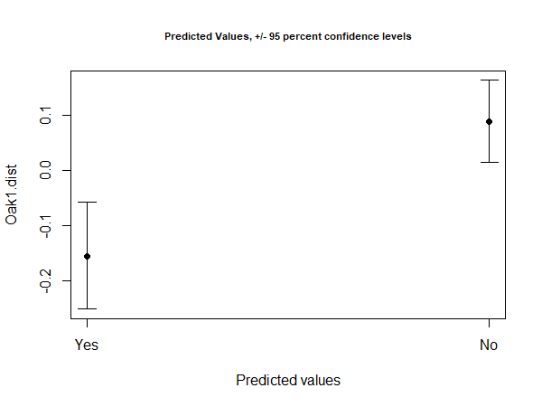
• x – an object of class ‘predict.lm.rrpp’.
• PC – whether to rotate the data and display the principal components. Default (FALSE) is to show the first two variables.  When TRUE, the points are shown maximizing the variation explained by these two dimensions.
• ellipse – whether to display confidence limits around the mean values. Default is to not do so.
• abscissa – vector of values used in predictions, to form horizontal axis of resulting plot.
• label – whether to add labels to the points. Default is to do so (TRUE).

plot(x = Oak.pred, PC = FALSE, ellipse = TRUE, abscissa = Oak.pred$grazing)

Application of RRPP to Semi-metric Distances

In the notes above, we demonstrated how RRPP could be used to analyze how species composition is affected by grazing status:

Oak.fit <- lm.rrpp(Oak1.dist ~ grazing, data = Oak.rrpp)

anova(Oak.fit)

Analysis of Variance, using Residual Randomization
Permutation procedure: Randomization of null model residuals 
Number of permutations: 1000 
Estimation method: Ordinary Least Squares 
Sums of Squares and Cross-products: Type I 
Effect sizes (Z) based on F distributions

          Df      SS      MS     Rsq      F      Z Pr(>F)   
grazing    1  1.0401 1.04009 0.04674 2.2063 3.0428  0.003 **
Residuals 45 21.2135 0.47141 0.95326                        
Total     46 22.2536                                        
---
Signif. codes:  0 ‘***’ 0.001 ‘**’ 0.01 ‘*’ 0.05 ‘.’ 0.1 ‘ ’ 1

Call: lm.rrpp(f1 = Oak1.dist ~ grazing, data = Oak.rrpp)

However, this analysis does not match the results of a PERMANOVA analysis using the default settings of adonis2():

grazing.result.adonis2 <- adonis2(Oak1.dist ~ grazing, data = Oak)

Permutation test for adonis under reduced model
Terms added sequentially (first to last)
Permutation: free
Number of permutations: 999

adonis2(formula = Oak1.dist ~ grazing, data = Oak)
         Df SumOfSqs      R2      F Pr(>F)    
grazing   1   0.6491 0.05598 2.6684  0.001 ***
Residual 45  10.9458 0.94402                  
Total    46  11.5949 1.00000                  
---
Signif. codes:  0 ‘***’ 0.001 ‘**’ 0.01 ‘*’ 0.05 ‘.’ 0.1 ‘ ’ 1

Note the difference in the total SS within the two analyses (I’ve made them bold) – 22.2536 vs. 11.5949.  All other differences between these analyses follow from this difference.

Michael Collyer, the lead author of RRPP, indicates that this discrepancy is because the Bray-Curtis distance measure is semi-metric.  This means that it does not satisfy the triangle inequality and cannot be perfectly mapped in a Euclidean space.  One way that this is demonstrated is through negative eigenvalues in a Principal Coordinate Analysis (PCoA) – these can be calculated mathematically but are problematic for interpretation.

RRPP automatically adjusts values, forcing semi-metric distances to behave as if they were metric.  We can avoid these values in adonis2() by including a correction factor which forces the distance matrix to be metric (i.e., to satisfy the triangle inequality).  Having done so, the ANOVA table from adonis2() is identical to that from lm.rrpp().

grazing.result.adonis2a <- adonis2(Oak1.dist ~ grazing, data = Oak, add = "cailliez")

Permutation test for adonis under reduced model
Terms added sequentially (first to last)
Permutation: free
Number of permutations: 999

adonis2(formula = Oak1.dist ~ grazing, data = Oak, add = "cailliez")
         Df SumOfSqs      R2      F Pr(>F)   
grazing   1   1.0401 0.04674 2.2063  0.002 **
Residual 45  21.2135 0.95326                 
Total    46  22.2536 1.00000                 
---
Signif. codes:  0 ‘***’ 0.001 ‘**’ 0.01 ‘*’ 0.05 ‘.’ 0.1 ‘ ’ 1

In this case, the effect of grazing remains significant but there is no assurance that that will always be the case.

Whether this correction is acceptable will depend on your research foci.  I’m not aware of any studies assessing the effect of this correction on statistical conclusions.

Conclusions

RRPP is widely applicable, particularly for datasets where it is appropriate to represent the data using a metric measure such as Euclidean distance.  RRPP includes features that are unavailable in other techniques, such as the ability to test random effects and to use many of the follow-up techniques that are available to conventional (univariate) linear models.

Some recent papers that used this technique (e.g., Kucuk et al. 2023) described their approach as doing a PERMANOVA using RRPP::lm.rrpp().  This language highlights the similarity between RRPP and PERMANOVA.

However, PERMANOVA (vegan::adonis2()) provides some additional control when analyzing semi-metric measures.  When semi-metric dissimilarity measures are used, RRPP automatically adjusts the dissimilarities so that they behave as if they are metric.  Doing so alters the relationships between the data matrix and the dissimilarity matrix: the dissimilarities are not simply based on the data in two sample units but on those data plus some adjustments to make the set of dissimilarities ‘behave’.  However, it is unclear how much of an effect this has on the conclusions of an analysis.

References

Collyer, M.L., and D.C. Adams. 2018. RRPP: an R package for fitting linear models to high-dimensional data using residual randomization. Methods in Ecology and Evolution 9:1772-1779.

Gagnon, E., L. Baldaszti, P. Moonlight, S. Knapp, C.E.R. Lehmann, and T. Särkinen. 2023. Functional and ecological diversification of underground organs in Solanum. Frontiers in Genetics 14:1231413.

Kucuk, R.A., B.J. Campbell, N.J. Lyon, E.A. Shelby, and M.S. Caterino. 2023. Gut bacteria of adult and larval Cotinis nitida Linnaeus (Coleoptera: Scarabaeidae) demonstrate community differences according to respective life stage and gut region. Frontiers in Microbiology 14:1185661.

Telemeco, R.S., and E.J. Gangloff. 2020. Analyzing stress as a multivariate phenotype. Integrative and Comparative Biology 60:70-78.