Introduction

Recall that ordinations are used for two primary purposes:

• Data reduction (i.e., reducing dimensionality)
• Visualization

Ordinations are not used for statistical tests – constrained ordinations blur the boundary between the two, though they don’t provide significance tests.  Instead, it is most helpful to think of all ordinations as visual support for the statistical tests that have been conducted.  They can also help generate hypotheses that are then investigated in future studies.

We noted at the start of this section that the ‘ideal’ ordination does not exist.  And, as you may have noticed from the readings (e.g., von Wehrden et al. 2009) and from your conversations with others, people have their own preferences about which ordination technique is preferred.  In my opinion, the appropriate ordination technique is the one whose assumptions your data most closely correspond to.

Here, I briefly review the assumptions and perceived pros and cons of the techniques that we’ve covered.

Eigenanalysis Techniques

PCA, CA, and related ordinations are based on eigenanalysis techniques:

• Based on the sample unit × species data matrix
• One eigenvalue per axis, with axes explaining declining proportions of the variance
• Each eigenvalue has associated eigenvectors
• The score for each sample unit along an axis is the sum of the products of the loadings (elements in the eigenvector) and variables (species).

PCA

PCA has the most restrictive assumptions (Euclidean distance measure, multivariate normality, linear relationships among variables) but is also the foundational ordination technique.  It is highly appropriate for some types of data, such as morphological/physiological data (e.g., Summerville et al. 2006) and LiDAR data (e.g., Kane et al. 2010), but is inappropriate for community-level data (Minchin 1987; Legendre & Legendre 2012). 

Other situations where PCA is particularly useful include:

• Translating and rotating data, as in the adjustments to the final solution in some NMDS ordinations, including metaMDS().  Note that, in this scenario, we keep all axes and therefore do not reduce the dimensionality.  As a result, the only effect of this procedure is to efficiently organize the data points in a configuration that can ease interpretation.
• Combining correlated variables to reduce the dimensionality of a dataset.  One or more of the resulting principal components can then be used as covariates in subsequent analyses (e.g., Haugo et al. 2011).

CA, DCA, and CCA

CA and related techniques have assumptions that are difficult to justify for community-level data (chi-square distance measure, unimodal species response curves).  They plot sample units and species on the same graph (a biplot), but the interpretation of these points may not be straight-forward.  For example, species on the edges of the scatter plot may be rare and those in the center may be unrelated to the axes, so the focus should be on species at intermediate distances from the centroid.  In addition, there’s the arch effect that shows up in CA (and can also occur in PCA and CCA).  Some folks advocate for DCA (Šmilauer & Lepš 2014) while others strongly advocate against it (e.g., McCune & Grace 2002; Gotelli & Ellison 2004).

Distance-based Techniques

NMDS

NMDS “preserves the rank order of the inter-point dissimilarities as well as possible within the constraints of a small number of dimensions” (Anderson et al. 2008, p. 105).  It has the least restrictive assumptions (any distance measure, no assumptions about shape of species response curves).

NMDS doesn’t provide quite the same types of information as other techniques – particularly because the axes have no direct meaning.  The user has to choose the number of dimensions, which can sound arbitrary or intimidating.  However, analyses can be rerun with different dimensions to identify the effect of dimensionality on stress.  And, the procedure is computationally intensive, though this concern is diminishing as computing power increases.  Species can be located in the ordination space using a different method than CA and DCA, though the same criticisms of such species scores apply.

PCoA

PCoA has parallels to both PCA and NMDS.  It is somewhat more restrictive than NMDS because it relates the distances in ordination space to the actual distances in the distance matrix (not the ranks of the distances).  However, PCoA has the flexibility that it can be used with any distance measure while projecting the points onto axes like PCA.  It is conceptually more similar to PERMANOVA than any of the other indirect gradient analysis techniques covered here.

PCoA is the default method for identifying the initial starting coordinates of a NMDS and for expressing sample unit locations in a Euclidean space in PERMDISP.

Constrained or Direct Gradient Analysis Techniques

Constrained techniques (CCA, RDA, dbRDA) are amalgamations or extensions of the other techniques.  They assume that you understand – a priori – the controlling gradient in your ecosystem.  Variability that is not related to the chosen environmental variables is ‘ignored’ (actually, it’s deferred to the unconstrained eigenvalues).

CCA makes the same assumptions as CA and DCA about the appropriateness of the chi-square distance measure, etc. (though I see it frequently in the literature, perhaps because it is an older technique).

RDA is appropriate if Euclidean distances are reasonable for your data, while dbRDA is appropriate with any distance measure.  Both of these techniques are amalgamations of other techniques.

One instance where RDA or dbRDA can be useful is as a follow-up to a statistical analysis in which you have identified an explanatory variable that relates to composition.  For example, dbRDA “will display a cloud of multivariate points by reference to a specific a priori hypothesis” (Anderson & Willis 2003, p. 511).  These techniques can be applied to data expressed with the same distance measure as was used in analysis, and will illustrate the differences due to the explanatory variables as strongly as possible.  See the following section for an example of this.

Different Views of the Same Point Cloud: Comparing Ordinations

Ordinations are often used with complex multivariate data.  The high dimensionality of these data implies that there are many ways to view them – imagine looking at a cloud of data points from different perspectives.  Furthermore, because ordinations are not statistical tests, it is appropriate to explore your data in different ways.  Let’s illustrate this by visualizing the relationship between grazing status and community composition in two complementary ways:

• Using NMDS to see differences between grazing treatments within the context of the ‘overall’ variability in composition
• Using dbRDA to see the maximal distinction between the grazing treatments

We’ll focus on the relationship between grazing history – the combination of current grazing status (GrazCurr) and past grazing status (GrazPast) – and the Oak1 response matrix.

Use the load.oak.data.R script to load and make initial adjustments to the oak plant community dataset.  The resulting Oak1 object contains abundances of the 103 most abundant species, each relativized by its maxima, while Oak_explan contains the potential explanatory variables.

source("scripts/load.oak.data.R")

Combine the two elements of grazing history together in a single column within Oak_explan (the object containing the explanatory variables).  For later use, I will also create a column containing the stand ID.

Oak_explan <- Oak_explan %>%
unite(col = Grazing, c(GrazPast, GrazCurr), remove = FALSE) %>%
mutate(Stand = rownames(Oak_explan))

PERMANOVA

Test whether plant community composition differs with respect to grazing status:

adonis2(Oak1 ~ Grazing,
data = Oak_explan,
distance = "bray")

Permutation test for adonis under reduced model
Terms added sequentially (first to last)
Permutation: free
Number of permutations: 999

adonis2(formula = Oak1 ~ Grazing, data = Oak_explan, distance = "bray")
         Df SumOfSqs      R2      F Pr(>F)   
Grazing   2   0.9095 0.07844 1.8725  0.007 **
Residual 44  10.6854 0.92156                 
Total    46  11.5949 1.00000                 
---
Signif. codes:  0 ‘***’ 0.001 ‘**’ 0.01 ‘*’ 0.05 ‘.’ 0.1 ‘ ’ 1

Yes, Grazing has a significant effect on plant community composition.

Conduct Ordinations (NMDS, dbRDA)

Conduct a NMDS of these data – :

set.seed(42)

Oak1_nmds <- metaMDS(comm = Oak1,
autotransform = FALSE,
k = 3)

I specified a 3-dimensional solution but did not adjust other NMDS arguments such as maxit, try, etc.  I also set the random number generator before running it to ensure that my output is repeatable.  Recall that this is unconstrained and does not incorporate grazing information.

Now, conduct a dbRDA relating oak plant community composition to grazing status:

Oak1_dbrda <- dbrda(Oak1 ~ Grazing,
data = Oak_explan,
distance = "bray")

print(Oak1_dbrda)

Call: dbrda(formula = Oak1 ~ Grazing, data = Oak_explan, distance
= "bray")

               Inertia Proportion Rank RealDims
Total         11.59490    1.00000              
Constrained    0.90946    0.07844    2        2
Unconstrained 10.68544    0.92156   44       33
Inertia is squared Bray distance 

Eigenvalues for constrained axes:
dbRDA1 dbRDA2 
0.7987 0.1108 

Eigenvalues for unconstrained axes:
  MDS1   MDS2   MDS3   MDS4   MDS5   MDS6   MDS7   MDS8 
1.5778 1.1950 1.0434 0.8402 0.7163 0.6529 0.5248 0.4470 
(Showing 8 of 44 unconstrained eigenvalues)

Compare the ANOVA table from the PERMANOVA and the summary of the dbRDA.  The SumOfSqs in the former is equivalent to the Inertia in the latter, and the proportion of variance associated with each term is identical in the two tables.

Organize Coordinates

Extract the coordinates from each ordination.  To graph the ordinations together, we need to combine their coordinates in a single object.  However, the coordinates are indexed in different ways and named differently for each ordination.  We will use a simple function to extract them, give them the same names (X, Y), and add columns distinguishing the type of ordination (Type) and identifying the stand (Stand).

Create function:

extract.coordinates <- function(xx, type) {
data.frame(X = xx[,1],
  Y = xx[,2],
  Stand = rownames(xx),
  Type = type)
}

Note that xx is the set of coordinates from the object produced by the ordination, not the object itself.

Apply this function to each ordination object:

Oak1_nmds_gg <- extract.coordinates(
xx = Oak1_nmds$points,
type = "NMDS")

Oak1_dbrda_gg <- extract.coordinates(
xx = summary(Oak1_dbrda)$sites,
type = "dbRDA")

Combine the two objects together:

NMDS_v_dbRDA <- rbind(Oak1_nmds_gg,
Oak1_dbrda_gg)

There are 94 rows in this object because each stand is represented twice – once from the NMDS and once from the dbRDA.

Add the grazing status to this object:

NMDS_v_dbRDA <- merge(x = NMDS_v_dbRDA,
by = "Stand",
y = Oak_explan[ , c("Stand", "Grazing")])

Create Graphs

Plot the ordinations beside each other:

ggplot(data = NMDS_v_dbRDA, aes(x = X, y = Y)) +
geom_point(aes(shape = Grazing, color = Grazing), size = 2)+
labs(shape = "Grazing", color = "Grazing") +
facet_wrap(vars(Type), scales = "free") +
theme_bw() +
theme(axis.line = element_line(),
  axis.ticks = element_blank(),
  axis.text = element_blank(),
  axis.title = element_blank())

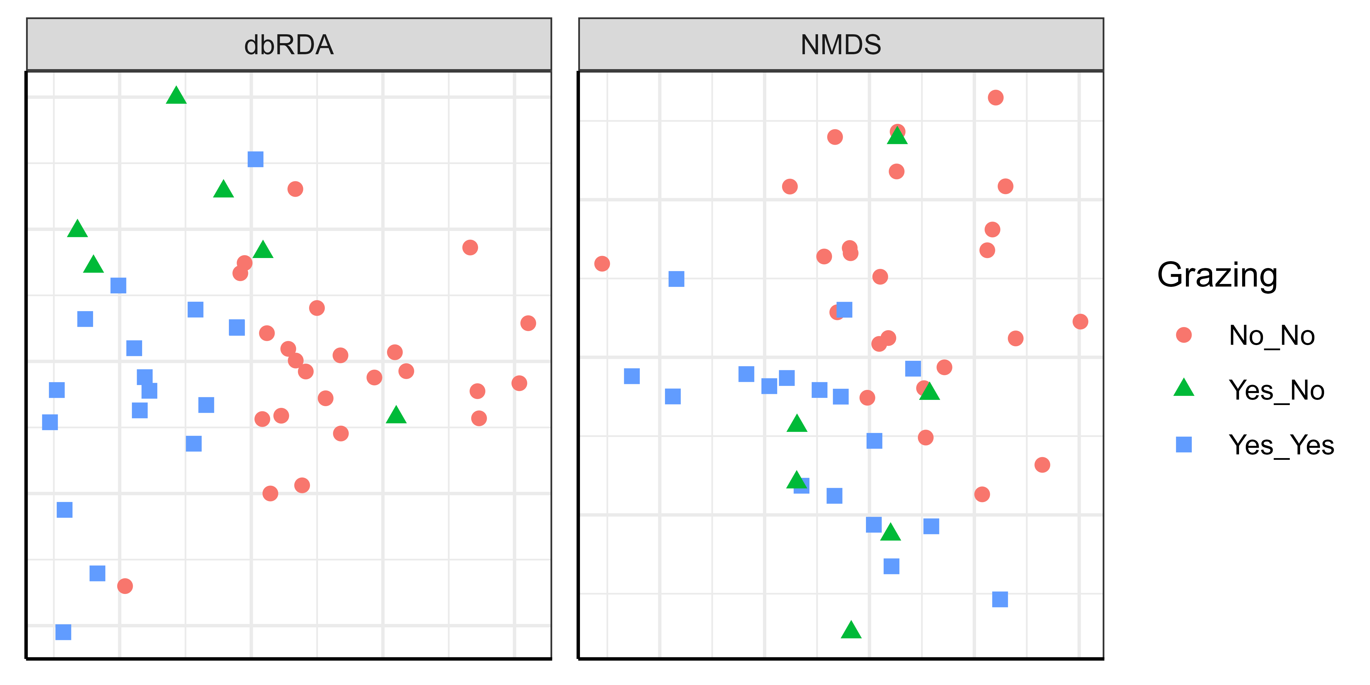
These two ordinations look different yet are based on exactly the same data!  Some notes:

• The grazing treatments are not in the same positions within each ordination, but this does not hinder interpretation.
• We did not include axis labels here.  It would be appropriate to do so for the dbRDA (including the amount of variation accounted for by each axis), but we generally would not do so for NMDS ordinations.
• In the NMDS ordination, sample units are located so that the data cloud accounts for as much of the variation in composition as possible.
  • The NMDS solution was rotated via PCA so that the axes account for diminishing amounts of the variation.
  • Grazing treatment was not incorporated into the ordination.  We superimposed it onto the ordination a posteriori by coding each sample unit by its grazing treatment.
  • Although grazing had a statistically significant effect on composition, it only accounted for 7.8% of the total variation in composition (see PERMANOVA results).  It therefore is not surprising that there is considerable overlap between the grazing treatments.
• In the dbRDA, we looked at the data cloud from the perspective that showed the maximal distinction between the grazing treatments.
  • There are three grazing treatments, so both visible axes are constrained.  The eigenvalues (summary(Oak1_dbrda)$cont) show that the first and second constrained axes account for 6.89% and 0.96%, respectively, of the variation in composition.  Together, these axes represent all possible variation that can be explained by grazing (i.e., 6.89 + 0.96 = 7.85%).
  • Note the ‘danger’ of misinterpreting the ordination … the axes have equal lengths here but we have to remember that the second axis accounts for a small amount of the total variation.  How much?  0.96 / 7.85 = 12.2% of the variation that can be explained by grazing status.  Therefore, the first axis is accounting for 87.7% of the variation that can be explained by grazing status.

Finally, please note that it is appropriate to consider, and even to display, different ordinations of the same data.  As evidenced here, these ordinations can give complementary insights into the structure of the data.

Procrustes Analysis

The above graphical comparison is visually striking, but what if we want to compare two ordinations statistically?  One way to do so is called Procrustes analysis (Peres-Neto & Jackson 2001).  (Aside: the story of Procrustes is a memorable one!)

Briefly, in Procrustes analysis we hold one ordination constant and then superimpose the other ordination onto it.  The superimposed ordination is rotated and scaled so that it corresponds as closely as possible to the other ordination.  The Procrustes statistic is the sum of squared differences between the positions of each sample unit in the two ordinations.  A helpful feature of Procrustes analysis is that it also permits the user to assess the alignment between individual observations, not just for the dataset as a whole (Peres-Neto & Jackson 2001).

Procrustes analysis can be conducted using the vegan::procrustes() function, or it can be conducted and the significance (non-randomness) of the relationship between the ordinations simultaneously assessed using the vegan::protest() function.

Let’s apply this to the two ordinations that we conducted above.  The two key arguments are the two ordinations to be compared; See the help file for other arguments in this function.  

procrustes.eg <- protest(Oak1_nmds, Oak1_dbrda)

print(procrustes.eg)

Call:
protest(X = Oak1_nmds, Y = Oak1_dbrda) 

Procrustes Sum of Squares (m12 squared):        0.6749 
Correlation in a symmetric Procrustes rotation: 0.5702 
Significance:  0.001 

Permutation: free
Number of permutations: 999

Note that we accepted the default of 999 unrestricted permutations.  More complex designs could be incorporated by restricting permutations using the how() function that we discussed in the context of group comparison tests.

The results indicate that there is a significant alignment between the two ordinations, although the correlation is somewhat low (0.57).

More helpful than the statistic itself is a visualization of the patterns:

plot(procrustes.eg)

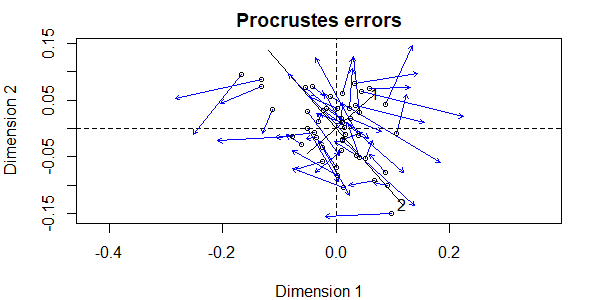
Notes:

• There are two sets of axes, one related to each ordination.
• The first set of axes (dashed lines) are from the first ordination that we specified – Oak1_nmds.
• The second set of axes (solid lines, with ‘1’ and ‘2’ labeling the two axes) are from the second ordination that we specified – Oak1_dbrda.  Note that axis 1 from this ordination is actually the smaller of the two axes when overlaid onto the NMDS ordination – this is an indication of how much the data cloud was rotated to align with the Grazing term.
• The symbols are the coordinates of the sample units in the rotated or second ordination (in this case, the dbRDA).
• Each sample unit has an associated blue arrow that points from its location in the second ordination to its location in the first ordination (the NMDS).  This highlights another benefit of this image – showing us which points in different ordinations represent the same sample unit.

Post-script: Negative Eigenvalues

The above comparison could also be made with RRPP as the statistical test.  However, lm.rrpp() automatically adjusts for negative eigenvalues – see the notes about this technique for details.  If you are going to visualize data that have been adjusted in this fashion during analysis, the ordination should also be adjusted in the same way.  If you don’t do this, the analysis and the visualization are not fully based on the same data.

Adjustments for negative eigenvalues are easily done in a dbRDA; see the  ‘add’ argument in the dbrda() function.

The metaMDS() function does not include an adjustment for negative eigenvalues.  One way to do so would be to conduct a PCoA with this adjustment, save all axes, and then conduct a NMDS on the PCoA dimensions.

Conclusions

There are a wide range of ordination techniques available, though they can be organized into broad themes.  In addition, some techniques are closely related (e.g., PCA is a special case of PCoA), and some techniques are amalgamations of others (e.g., dbRDA is a combination of PCoA, RDA, and PCA).

In my opinion, NMDS and dbRDA are some of the most robust techniques that we’ve covered.  A particularly appealing feature of these techniques is that they can be used to visualize a dataset using the distance measure as were used in a statistical analysis.  Furthermore, dbRDA follows the same logic as PERMANOVA.

The relative differences among some of these techniques are unclear; Anderson (2015) notes that techniques like NMDS and PCoA will tend to give similar results, and that far more important differences arise from decisions about data adjustments (transformations, standardizations) and which distance measure to use.

I’ve stressed that ordinations primarily are visualization tools.  They therefore are often most appropriately thought of in a supplementary role – for example, supporting a statistical analysis by demonstrating a statistically significant pattern that has been detected.

In some cases, ordinations can be very effective means of data reduction.  This is particularly true for PCA, where the principal components can be related to the original variables and can be analyzed independently even though the original variables were correlated with one another.

A few wise quotes to conclude:

“A biologist’s insight, experience, and knowledge of the literature are the most important tools for interpreting indirect gradient analysis” (source missing).

“… when the dust settles, if you’ve found a pattern in NMDS, you will probably find something similar with DCA/CCA and maybe even with PCA.  When you see someone’s presentation which contains a DCA ordination or CCA, there’s probably good information in it … and shouting, “Your ordination sucks, man!” probably won’t get you deep into an informative conversation.” (Mike Kearsley, 2003, unpublished).

References

Anderson, M.J., R.N. Gorley, and K.R. Clarke. 2008. PERMANOVA+ for PRIMER: guide to software and statistical methods. PRIMER-E Ltd, Plymouth, UK.

Anderson, M.J., and T.J. Willis. 2003. Canonical analysis of principal coordinates: a useful method of constrained ordination for ecology. Ecology 84:511-525.

Gotelli, N.J., and A.M. Ellison. 2004. A primer of ecological statistics. Sinauer, Sunderland, MA.

Haugo, R.D., C.B. Halpern, and J.D. Bakker. 2011. Landscape context and long-term tree influences shape the dynamics of forest-meadow ecotones in mountain ecosystems. Ecosphere 2:art91.

Kane, V.R., R.J. McGaughey, J.D. Bakker, R.F. Gersonde, J.A. Lutz, and J.F. Franklin. 2010. Comparisons between field- and LiDAR-based measures of stand structural complexity. Canadian Journal of Forest Research 40:761-773.

Legendre, P., and L. Legendre. 2012. Numerical ecology. Third English edition. Elsevier, Amsterdam, The Netherlands.

McCune, B., and J.B. Grace. 2002. Analysis of ecological communities. MjM Software Design, Gleneden Beach, OR.

Minchin, P.R. 1987. An evaluation of the relative robustness of techniques for ecological ordination. Vegetatio 69:89-107.

Peres-Neto, P.R., and D.A. Jackson. 2001. How well do multivariate data sets match? The advantages of a Procrustean superimposition approach over the Mantel test. Oecologia 129: 169-178.

Šmilauer, P., and J. Lepš. 2014. Multivariate analysis of ecological data using CANOCO 5. 2nd edition. Cambridge University Press, Cambridge, UK.

Summerville, K.S., C.J. Conoan, and R.M. Steichen. 2006. Species traits as predictors of lepidopteran composition in restored and remnant tallgrass prairies. Ecological Applications 16:891-900.

von Wehrden, H., J. Hanspach, H. Bruelheide, and K. Wesche. 2009. Pluralism and diversity: trends in the use and application of ordination methods 1990-2007. Journal of Vegetation Science 20:695-705.