
Group Comparisons
16 Permutation Tests
Learning Objectives
To explore the theory behind permutation-based tests.
To illustrate how permutation tests can be conducted in R.
Key Packages
require(tidyverse)
Introduction
A statistical test involves the calculation of a test statistic followed by an assessment of how likely the calculated value of the test statistic would be if the data were randomly distributed. In the case of ANOVA, the test statistic is the F-statistic, and it is compared to the theoretical distribution of F-values with the same degrees of freedom.
We will consider a number of tests using a range of test statistics. However, there is no theoretical distribution for these test statistics. Rather, the distribution of the test statistic will be derived from the data. Generally, this reference distribution is generated by permuting (i.e., randomly reordering) the group identities, recalculating the test statistic, saving that value, and repeating this process many times (Legendre & Legendre 2012).
If the patterns observed in the data are unlikely to have arisen by chance, then the actual value of the test statistic should differ from the set of values obtained from the permutations.
Key Takeaways
The number of sample units directly affects the number of permutations.
Some permutations are functionally equivalent, so there are fewer combinations for a given sample size.
Number of Permutations (and Combinations)
The number of samples directly affects the number of possible permutations and combinations.
A permutation is a re-ordering of the sample units. From a total of n sample units, the number of possible permutations (P) is:
[latex]P = n![/latex]
The number of permutations rises rapidly with sample size – see the table below. To explore this, enumerate the permutations of the letters {a, b, C, D}. There are four values, so the number of permutations is:
[latex]P = n! = 4 \cdot 3 \cdot 2 \cdot 1 = 24[/latex]
Assume that the letters {a, b, C, D} represent sample units, with lower and upper cases representing different groups. In other words, the first two sample units are in one group and the last two are in the other group. One permutation of these letters is {a, C, b, D}. In this permutation, we assign the first and third sample units to one group and the second and fourth sample units to the other group. Note that this ‘assignment’ is temporary and only for the purpose of this permutation.
When we think about group comparisons, it is helpful to recognize that some permutations are functionally equivalent. For example, consider the permutations {a, C, b, D} and {C, a, D, b}. In both permutations, the first and third sample units are assigned to one group and the second and fourth sample units are assigned to the other group. These permutations represent the same combination. A combination is a unique set of sample units, irrespective of sample order within each set. The number of combinations (C) of size r is:
[latex]C_{r}^{n} = \frac{n!}{r! (n - r)!}[/latex]
(this equation is from Burt & Barber 1996). This is for equally-sized groups; the calculations are more complicated for groups of different sizes.
For our simple example of four sample units, there are
[latex]C_{r}^{n} = \frac{n!}{r! (n - r)!} = \frac{4!}{2! (4 - 2)!} = \frac{4 \cdot 3 \cdot 2 \cdot 1}{2 \cdot 1 (2 \cdot 1)} = 6[/latex]
The following table shows how the number of permutations and combinations (into two equally-sized groups) rises rapidly with the number of sample units.
| Samples (n) | Permutations (P) | Samples per group (r) | Combinations (C) |
| 4 | 24 | 2 | 6 |
| 8 | 40,320 | 4 | 70 |
| 12 | 479,001,600 | 6 | 924 |
| 16 | 2.1 × 10¹³ | 8 | 12,870 |
| 20 | 2.4 × 10¹⁸ | 10 | 184,756 |
| 24 | 6.2 × 10²³ | 12 | 2,704,156 |
| 28 | 3.0 × 1029 | 14 | 40,116,600 |
| 32 | 2.6 × 1035 | 16 | 601,080,390 |
| 36 | 3.7 × 1041 | 18 | 9,075,135,300 |
| 40 | 8.2 × 1047 | 20 | 137,846,528,820 |
Probabilities
Permutation-based probabilities are calculated as the proportion of permutations in which the computed value of the test statistic is equal to or more extreme than the actual value. This calculation can be made with any number of permutations, though it is easier to do so mentally if the denominator is a multiple of ten, such as 1,000.
The actual sequence of group identities is one of the possible permutations and therefore is included in the denominator of the probability calculation. This is why it is common to do, for example, 999 permutations – once the actual sequence is included, the denominator of the probability calculation is 1,000.
The minimum possible P-value is partly a function of the number of permutations. For example, consider a scenario in which the test statistic is larger when calculated with the real data than when calculated for any of the permutations. If we had only done 9 permutations, we would calculate
[latex]P = \frac{1}{9 + 1} = 0.1[/latex]
However, if we had done 999 permutations, we would calculate
[latex]P = \frac{1}{999 + 1} = 0.001[/latex]
Would it make sense to declare that the effect is significant in the second case but not in the first?
For studies with reasonably large sample sizes, there are many more permutations than we can reasonably consider. For example, there are 8.2 × 1047 permutations of 40 samples as reported in the above table. If we considered one every millisecond (i.e., 1000 per second), it would still take us 2.6 × 1037 years to consider them all!
Given the large number of possible permutations, we usually assess only a small fraction of them. This means that permutation-based probability estimates are subject to sampling error and vary from run to run. The variation between runs declines as the number of permutations increases; more permutations will result in more consistent estimates of the probability associated with a test statistic. Legendre & Legendre (2012) offer the following recommendations about how many permutations to compute:
- Use 500 to 1000 permutations during exploratory data analyses
- Rerun with an increased number of permutations if the computed probability is close to the preselected significance level (either above or below)
- Use more permutations (~10,000) for final, published results
The system.time() function can be used to measure how long a series of permutations requires.
Key Takeaways
The statistical significance of a permutation-based test is the proportion of permutations in which the computed value of the test statistic is equal to or more extreme than the actual value.
The actual value of the test statistic is unaffected by the number of permutations.
It’s ok to use small numbers of permutations during exploratory analyses, but use a large number (~10,000) for final analyses.
Exchangeable Units
I mentioned two assumptions of ANOVA / MANOVA in that chapter; a third foundational assumption of both techniques is that the sample units are independent. Analyses may be suspect when this is not the case or when the lack of independence is not properly accounted for. Failure to account for lack of independence is a type of pseudoreplication (Hurlbert 1984).
The assumption of independence also applies for permutation tests – it is what justifies exchangeability in a permutation test. This means that it is possible to analyze a permutation-based test incorrectly. Permutations need to be restricted when sample units are not exchangeable. The correct way of permuting data depends on the structure of the study and the hypotheses being tested. The basic idea is that the exchangeable units that would form the denominator when testing a term in a conventional ANOVA are those that should be permuted during a permutation test of that term.
Questions about independence and exchangeability are particularly pertinent for data obtained from complex designs that include multiple explanatory variables simultaneously. See Anderson & ter Braak (2003), Anderson et al. (2008), and Legendre & Legendre (2012) for details on how to identify the correct exchangeable units for a permutation test.
For example, in a split-plot design one factor can be applied to whole plots and another factor to split plots (i.e., within the whole plots). Each of these factors would require a different error term.
- Analyses of the whole plot factor use the unexplained variation among whole plots as the error term. This is evident in the fact that the df for the whole plot error term is based on the number of whole plots, regardless of how many measurements were made within them. In a permutation test, variation among whole plots is assessed by restricting permutations such that all observations from the same whole plot are permuted together. Variation within whole plots is ignored when analyzing whole plot effects.
- Analyses of the split-plot factor use the residual as the error term and therefore do not require restricted permutations. However, they do require the inclusion of a term that uniquely identifies each whole plot so that the variation among whole plots is accounted for. Doing so allows the analysis to focus on the variation within whole plots. If a model included interactions with the split-plot factor, these would also be tested at this scale.
More information on this topic is provided in the chapter about complex models.
Implementation in R
The sample() function can be used to permute data. If needed, you can use the size argument to create a subset, and the replace argument to specify whether to sample with replacement (by default, this is FALSE).
The vegan package, drawing on the permute package, includes a number of options for conducting permutations. This topic is explained in more detail in the chapters about controlling permutations and restricting permutations.
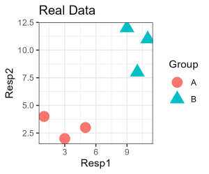
Simple Example, Graphically
Since our simple example only has two response variables, it is easily visualized:
library(tidyverse)
ggplot(data = perm.eg, aes(x = Resp1, y = Resp2)) +
geom_point(aes(colour = Group, shape = Group), size = 5) +
labs(title = "Real Data") +
theme_bw()
ggsave("graphics/main.png", width = 3, height = 2.5, units = "in", dpi = 300)(did you notice that we saved the image, and where we saved it?)
To conduct a permutation, we can permute either the grouping factor or the data. Can you see why these are equivalent? We would not permute both at the same time … do you see why that is?
We’ll permute the grouping factor:
perm.eg$perm1 <- sample(perm.eg$Group)
We’ve added the permutation as a new column within the perm.eg object. View the object to compare the permutation with the original grouping factor. Note that the number of occurrences of each group remains the same in permutations as in the original.
Let’s visualize this permutation of the data. We can use the same code as above with a few changes:
- Name of column identifying the groups used for
colourandshapewithingeom_point(). - Title of figure
- Name of file to which image is saved
ggplot(data = perm.eg, aes(x = Resp1, y = Resp2)) +
geom_point(aes(colour = perm1, shape = perm1), size = 5) +
labs(title = "Permutation 1") +
theme_bw()
ggsave("graphics/perm1.png", width = 3, height = 2.5, units = "in", dpi = 300)

It is possible but somewhat unlikely that the group identities in your graph match this one. Be sure you understand why!
Simple Example, Distance Matrix
Analyses will be based on the distance matrix so let’s consider this. Here it is:
Resp.dist <- perm.eg |>
dplyr::select(Resp1, Resp2) |>
dist()

round(Resp.dist, 3)
| Plot1 | Plot2 | Plot3 | Plot4 | Plot5 | |
| Plot2 | 2.828 | ||||
| Plot3 | 4.123 | 2.236 | |||
| Plot4 | 11.314 | 11.662 | 9.849 | ||
| Plot5 | 9.849 | 9.220 | 7.071 | 4.123 | |
| Plot6 | 12.207 | 12.042 | 10.000 | 2.236 | 3.162 |
Group identity was not part of the distance matrix calculation. This means that permuting the group identities doesn’t change the distance matrix itself.
Permuting group identities does change which distances connect sample units assigned to the same group. For example, plots 1, 2, and 3 are all in group A in our real data but plots 2, 4, and 6 were assigned to group A in Permutation 1 above.
Note: To keep our example simple, we did not relativize the data and calculated Euclidean distances. These decisions do not affect the permutations but, as discussed before, these decisions should be based on the nature of your data and your research questions.
Grazing Example
Our grouping factor for this example is current grazing status (Yes, No). The sample() function can also be applied here:
sample(grazing)
We’ll use this example in more detail in upcoming chapters.
References
Anderson, M.J., R.N. Gorley, and K.R. Clarke. 2008. PERMANOVA+ for PRIMER: guide to software and statistical methods. PRIMER-E Ltd, Plymouth Marine Laboratory, Plymouth, UK. 214 p.
Anderson, M.J., and C.J.F. ter Braak. 2003. Permutation tests for multi-factorial analysis of variance. Journal of Statistical Computation and Simulation 73:85-113.
Burt, J.E., and G.M. Barber. 1996. Elementary Statistics for Geographers. 2nd edition. Guilford Publications.
Hurlbert, S.H. 1984. Pseudoreplication and the design of ecological field experiments. Ecological Monographs 54:187-211.
Legendre, P., and L. Legendre. 2012. Numerical ecology. 3rd English edition. Elsevier, Amsterdam, The Netherlands.
Media Attributions
- main
- perm1
