Introduction

A univariate regression tree (URT) relates a single response variable to one or more explanatory variables through a series of binary splits. De’ath (2002) extended URTs to multivariate data.  A multivariate regression tree (MRT) obviously requires a multivariate response.

More importantly, a MRT also requires that impurity be redefined in a multivariate sense.  Three ways are available:

• Sums of squares MRT (SS-MRT) – “Geometrically, this is simply the sum of squared Euclidean distances of sites about the node centroid.  Each split minimizes the sums of squared distances (SSD) of sites from the centroids of the nodes to which they belong.  Equivalently, this maximizes the SSD between the node centroids” (De’ath 2002, p. 1107).
• Additive MRT – uses other sums of squares formulas, such as the sums of absolute deviations about the median.
• Distance-based MRT (db-MRT) – impurity is defined as the sum of within-group squared distances (as in PERMANOVA).  This can be applied to any distance measure – including semimetric measures – and therefore is more general than the other ways of defining multivariate impurity.  For example, it is directly applicable to community-level data.  A db-MRT with Euclidean distances is exactly equivalent to a SS-MRT.

See Section 4.11 of Borcard et al. (2018) for a nice summary of MRTs.

The mvpart() function is built to handle both URTs and MRTs.  Concepts such as pruning and cross-validation are the same with both types of data.  However, not all arguments work with all methods of calculating impurity.

Each leaf/terminal node of a MRT can be characterized by:

• the multivariate mean of its observations (e.g., mean abundance of each species on the plots in that leaf/terminal node)
• the number of observations (plots)
• the environmental variables that distinguish it from others
• the species that are strongly associated with it

Of course, we’re dealing with multivariate data here so the other analysis considerations that we’ve discussed throughout the course still apply:

• data transformation
• data standardization
• choice of distance measure (for db-MRT)

These choices can affect the results.  For example, the SS-MRT reported by De’ath (2002; his Figure 2) differs from ours below because he used a different type of standardization.  This is illustrated below.

MRTs in R

We’ll use the same spider data that were used to introduce URTs.  However, rather than exploring the abundance of one spider species, we’ll consider the composition of the spider community as a function of the measured environmental variables.

The spider abundances are already on a common scale (0-9; ordinal) so we won’t relativize them.  We begin by saving the data as a matrix:

spider.std <- data.matrix(spider[,1:12])

Sums of squares MRT (SS-MRT)

Now, we’ll perform a SS-MRT on the compositional data using Euclidean distances:

SSMRT.spider <- mvpart(spider.std ~ .,
data = env,
xv = "pick",
xvmult = 100,
control = rpart.control(xval = nrow(spider)/2),
plot.add = TRUE,
all.leaves = TRUE,
dissim = "euc")

The bold font indicates the two items that changed from the last URT that we conducted (Troc.terr.xv):

• The left-hand side of the formula to be tested.  Note that this is of class matrix; mvpart() automatically uses method = "mrt" for objects of this class.  If we wanted to be more explicit about this, we could have added the method argument to the function.  By analogy, when we considered URTs we did not specify a method and mvpart() automatically used method = "anova".
• The argument dissim = "euc" was added.

We once again set xv = "pick" so that we could select the best tree interactively.  I don’t show that here, but in this case I selected a tree of size 5.

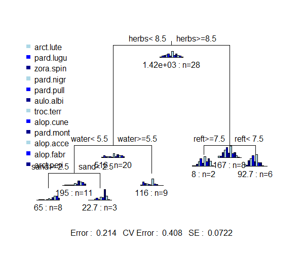
The graph of a SS-MRT tree includes box plots showing the relative abundance of each species in each group.  Note that these look similar to – but are definitely different from – the histograms that are sometimes provided in an URT.

Interpretation of the nodes and the explanatory variables chosen for each split are the same as for a URT.

The quantitative summary also has a very similar format to that for a URT:

summary(SSMRT.spider)

Call:
mvpart(form = spider.std ~ ., data = env, xv = "pick", xvmult = 100, 
    plot.add = TRUE, all.leaves = TRUE, control = rpart.control(xval = nrow(spider)/2), 
    dissim = "euc")
  n= 28 

          CP nsplit rel error
1 0.51864091      0 1.0000000
2 0.14489010      1 0.4813591
3 0.07537481      2 0.3364690
4 0.04678068      3 0.2610942
5 0.03530100      4 0.2143135
     xerror       xstd
1 1.0769716 0.12649336
2 0.5631391 0.07505089
3 0.4317718 0.07445582
4 0.4252404 0.07684907
5 0.4080949 0.07224169

Node number 1: 28 observations,    complexity param=0.5186409
  Means=0.3571,1.179,1.536,1.964,2.5,1.179,4.5,1.393,2.5,1.5,0.9286,0.4286, Summed MSE=50.64158 
  left son=2 (20 obs) right son=3 (8 obs)
  Primary splits:
      herbs < 8.5 to the left,  improve=0.5186409, (0 missing)
      water < 5.5 to the left,  improve=0.3015809, (0 missing)
      moss  < 6   to the right, improve=0.2483042, (0 missing)
      reft  < 7.5 to the right, improve=0.2123679, (0 missing)
      sand  < 5.5 to the right, improve=0.2008664, (0 missing)

Node number 2: 20 observations,    complexity param=0.1448901
  Means=0.1,1.3,0.75,0.6,0.5,0.3,2.9,0.8,2.1,1.5,1.2,0.6, Summed MSE=25.7775 
  left son=4 (11 obs) right son=5 (9 obs)
  Primary splits:
      water < 5.5 to the left,  improve=0.3985045, (0 missing)
      twigs < 3.5 to the left,  improve=0.3985045, (0 missing)
      reft  < 3.5 to the right, improve=0.3985045, (0 missing)
      moss  < 6   to the right, improve=0.3518347, (0 missing)
      herbs < 6.5 to the left,  improve=0.2054174, (0 missing)

Node number 3: 8 observations,    complexity param=0.04678068
  Means=1,0.875,3.5,5.375,7.5,3.375,8.5,2.875,3.5,1.5,0.25,0, Summed MSE=20.875 
  left son=6 (2 obs) right son=7 (6 obs)
  Primary splits:
      reft  < 7.5 to the right, improve=0.39720560, (0 missing)
      moss  < 1.5 to the right, improve=0.34610780, (0 missing)
      water < 7   to the left,  improve=0.20159680, (0 missing)
      twigs < 1.5 to the right, improve=0.06986028, (0 missing)

Node number 4: 11 observations,    complexity param=0.07537481
  Means=0,0.1818,0.1818,0.3636,0.3636,0.1818,1.364,0.5455,3.364,2.727,2.182,1.091, Summed MSE=17.68595 
  left son=8 (8 obs) right son=9 (3 obs)
  Primary splits:
      sand  < 2.5 to the right, improve=0.54937690, (0 missing)
      water < 3.5 to the left,  improve=0.54454270, (0 missing)
      herbs < 6.5 to the left,  improve=0.43971960, (0 missing)
      reft  < 8.5 to the right, improve=0.20948210, (0 missing)
      moss  < 5.5 to the right, improve=0.09589823, (0 missing)

Node number 5: 9 observations
  Means=0.2222,2.667,1.444,0.8889,0.6667,0.4444,4.778,1.111,0.5556,0,0,0, Summed MSE=12.83951 

Node number 6: 2 observations
  Means=0.5,0.5,1.5,3.5,6,2.5,7.5,3.5,6,4,0.5,0, Summed MSE=4 

Node number 7: 6 observations
  Means=1.167,1,4.167,6,8,3.667,8.833,2.667,2.667,0.6667,0.1667,0, Summed MSE=15.44444 

Node number 8: 8 observations
  Means=0,0.25,0.25,0.25,0,0.125,1.125,0.125,1.75,2.75,2.875,1.5, Summed MSE=8.125 

Node number 9: 3 observations
  Means=0,0,0,0.6667,1.333,0.3333,2,1.667,7.667,2.667,0.3333,0, Summed MSE=7.555556 

Note that the mean abundance of each species is reported for each node – these are the data that are graphed to produce the bar plots in the above graphic.  The order of the species is not reported – you have to refer to the response matrix to determine which is which.

For each split, all possible breakpoints for all specified potential explanatory variables were evaluated and the variable and its breakpoint that most strongly separates the data into two groups is identified.  Other variables and their optimal breakpoints are shown as well.

PS: De’ath (2002) used SS-MRT but reported a different result in his Figure 2 for the multivariate analysis of the spider community.  Mike Marsh and Gavin Simpson determined that the difference is because De’ath standardized the data so that the rows and columns summed to 1.  Here’s code to do so:

spider.std1 <- scaler(spider[ , 1:12], col="mean1", row="mean1")

spider.mrt1 <- mvpart(spider.std1 ~ water + sand + moss + reft + twigs + herbs, data = env, xv = "pick")

Choose a tree of size 4 to replicate his result.

Distance-based MRT (db-MRT)

We can compare the above SS-MRT with the results of a db-MRT using Euclidean distances.  My testing suggests that mvpart() has issues with the distance matrices produced by some other functions, so we will use gdist(), the function provided within the mvpart package.  In addition, we have to store the full symmetric distance matrix (not just the lower triangle); we do so via the argument full = TRUE.

spider.euc <- gdist(spider.std,
method = "euclidean",
full = TRUE)

dbMRT.spider <- mvpart(spider.euc ~ .,
data = env,
xv = "pick",
xvmult = 100,
control =rpart.control(xval = nrow(spider)/2),
plot.add = TRUE,
all.leaves = TRUE)

For illustration purposes, I again chose a tree of size 5.

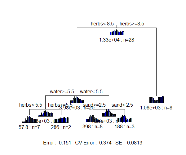
One important difference between the graphical representation of these trees: in SSMRT.spider, the bar plots are the individual species, whereas in dbMRT.spider, the bar plots are the distances between sample units (note that there are a lot more of them, and that these bar plots are not so useful).

We’ve talked throughout the course about how Euclidean distances are not generally appropriate for compositional data.  With distance-based MRTs, we can also use other distance measures such as Bray-Curtis:

spider.bc <- gdist(spider.std,
method = "bray",
full = TRUE)

dbMRT.spider <- mvpart(spider.bc ~ .,
data = env,
xv = "pick", xvmult = 100,
control =rpart.control(xval = nrow(spider)/2),
plot.add = TRUE,
all.leaves = TRUE)

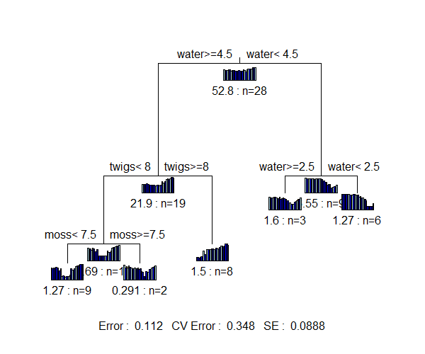
Trees based on different distance measures can be directly compared.  Comparing the MRTs based on Euclidean and Bray-Curtis distances:

• The MRT based on Bray-Curtis distances resulted in a slightly smaller cross-validated relative error (0.348) than that based on Euclidean distances (0.374).  Other datasets may have different conclusions.
• Different variables form the basis of the splits in these trees – herbs, water, and sand for the Euclidean MRT vs. water, twigs, and moss for the Bray-Curtis MRT.
• I specified trees of the same size (5 terminal nodes) in both MRTs so I could more easily compare them, but the optimal size may differ among trees.
• Even when the trees are the same size, if they’re split on the basis of different variables and breakpoints then the size of each terminal node can differ and so can the identity of the samples within each terminal node.

Interpretation of a MRT

In a MRT, we generally focus on the leaves (terminal nodes).  Interpretation of a MRT can be based on various tools and techniques:

• Recognize that splits at the top of the tree are more important than those that occur near the leaves.
• Species abundances can be graphed onto the regression tree.
• The explained variance at each split for each species can be tabulated.  One way to use these data is to identify species that most strongly determine the splits of the tree.
• The sample units can be ordinated (plotted in a low-dimensional space) and overlaid with information such as leaf (terminal node) identity, species abundance, etc.
• Indicator Species Analysis (ISA) can be used to identify the species that characterize each group.  This can be done in several ways:
  • Two examples – the MRT() function and the indicspecies package (De Cáceres & Legendre 2009; De Cáceres et al. 2010) – are illustrated below.  See here for more information about ISA.
  • Borcard et al. (2018; Section 4.12.4) discuss another way to do an ISA.
  • A slightly different approach is to relate species abundances directly to the explanatory variables – this can be done with continuously distributed variables using Threshold Indicator Taxa ANalysis (TITAN) in the TITAN2 package (Baker & King 2010).  See here for more information about TITAN.
• The resulting groups can be compared with the solution from an unconstrained cluster analysis:
  • If the unconstrained cluster analysis accounts for more of the species variation, unobserved factors (not included in the matrix of environmental variables) may be important.
  • If the two methods explain similar amounts of species variation, it is likely that important environmental variables (or their surrogates) have been identified.
  • If unconstrained clustering is weak but species – environment relationships are strong, the MRT may detect groups the unconstrained cluster analysis does not.

How to Use the Groups from a MRT

We begin by saving the group identity of each sample unit as identified in the terminal nodes of our tree.  In this case, we’ll use the result of the Bray-Curtis dissimilarity matrix:

spider$g5 <- dbMRT.spider$where

Alternatively, we could script the group assignments based on the regression tree.  This can be helpful if we want to give the groups more informative names, for example.  For each group, we simply work our way down through the tree.  The case_when() function is very helpful here rather than using a series of ifelse() statements:

spider <- spider %>%
mutate(g5.alt = case_when(
water >= 4.5 & twigs < 8 & moss < 7.5 ~ "A",
  water >= 4.5 & twigs < 8 & moss >= 7.5 ~ "B",
water >= 4.5 & twigs >= 8 ~ "C",
  water < 4.5 & water >= 2.5 ~ "D",
water < 4.5 & water < 2.5 ~ "E"))

Note that I’ve simply named the groups from left to right in the tree.  Comparing these two approaches:

table(spider$g5, spider$g5.alt)

    A B C D E
  4 9 0 0 0 0
  5 0 2 0 0 0
  6 0 0 8 0 0
  8 0 0 0 3 0
  9 0 0 0 0 6

The two approaches assign observations to the same groups, though I named the groups with letters while the summary reported the terminal node numbers.

As with the URT, we can use this index to subset or understand our data in different ways.  Two of these techniques are illustrated here.  These techniques could also be used with the groups identified through a cluster analysis, etc.

Summarizing Data For Each Group

Here, we’ll summarize the environmental data based on these group identities:

spider %>%
select(colnames(env), g5.alt) %>%
group_by(g5.alt) %>%
summarize(across(everything(), mean), .groups = "keep")

# A tibble: 5 × 7
# Groups:   g5.alt [5]
  g5.alt water  sand  moss  reft twigs herbs
  <chr>  <dbl> <dbl> <dbl> <dbl> <dbl> <dbl>
1 A       7.44 0.889  3.33  5     1.44  8.67
2 B       5    0      8.5   7.5   0     7   
3 C       7.75 0      1.25  0.75  9     3.12
4 D       3.67 5      6     7     0     6.67
5 E       0.5  6.83   7.83  8.5   0     4.17

The result is the mean value of each explanatory variable in each terminal node from the MRT.  Explanatory variables that were not selected to split the tree are probably of less interest – but could be important if the chosen variables were not in the model.

We could do the same type of summary for the response variables (species abundances).  See below for an example of how Indicator Species Analysis can be used to identify the group or set of groups with which each species is most strongly associated.

Overlay Groups Onto An Ordination

We can overlay the resulting groups onto an ordination.  We’ll illustrate this using a NMDS ordination:

library(vegan)

spider.NMDS <- metaMDS(spider.bc, k = 2, wascores = FALSE)

The coordinates of each plot are provided in the points aspect of this object, so let’s add them to the spider object:

spider2 <- data.frame(spider, spider.NMDS$points)

We’ll illustrate this using ggplot2, and we’ll make the symbol size proportional to the value of water (since that was the first variable selected in the db-MRT and thus is the most important explanatory variable distinguishing the groups):

ggplot(data = spider2, aes(x = MDS1, y = MDS2)) +
geom_point(aes(fill = g5.alt, size = water), shape = 21) +
labs(title = "Groups from regression tree", x = "", y = "", fill = "Group") +
scale_x_continuous(labels = NULL, breaks = NULL) +
scale_y_continuous(labels = NULL, breaks = NULL) +
theme_bw()

ggsave("graphics/spider_tree.png", width = 4, height = 3, units = "in", dpi = 300)

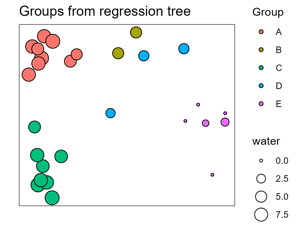
We’ll discuss ordinations soon, but for now I’ll note that this ordination is based entirely on the distance matrix derived from the response variables (species abundances).  In contrast, the tree and associated classification are based on the relationship between that same distance matrix and the explanatory variables.  Alignment between the ordination and the regression tree – observations that are close to one another in the ordination also being assigned to the same group in the MRT – is an indication that composition varies substantially with respect to water.  

In this graphic, point size relates to water, which was the basis for the first split in this tree and point color relates to the groups identified in the MRT.  Group E, those associated with the lowest values for water, are on one end of the ordination while groups with higher values for water are on the other end of the ordination.

The regression tree (shown above) indicates that twigs and moss are also important in distinguishing some groups, though we have not incorporated them into this image.

Explore Other Aspects of MRT Output

The MVPARTwrap package is not actively maintained and therefore has to be installed from github:

devtools::install_github("cran/MVPARTwrap", force = TRUE)

library(MVPARTwrap)

It includes the MRT() function, which is a wrapper that provides additional output from a MRT analysis.  Its usage is:

MRT(
obj,
percent,
species = NULL,
LABELS = FALSE,
...
)

The key arguments are:

• obj – the object to be summarized (class mvpart).
• percent – the minimum importance of a species.  Summary will highlight species that account for at least this much variance at a node.  Default not specified, but appears to be 10.
• species – a vector of species names.

The output includes:

• nodes – node numbers, in increasing order of contribution to explained variance.
• pourct – species contributions to explained variation (%) at each node.  Each row is a node, and each column is a species.  Note that this order is transposed from that in TABLE1 below.  In addition, the values here are percentages of the column totals from TABLE1.
• R2 – species contribution to explained variation at each node.  R² is equal to 1 minus the relative error.  Same information for each species as in TABLE1, but expressed as a proportion and in transposed order.
• RWHERE, LWHERE – a list of vectors containing the row numbers of objects or left or right side of each node.
• TABLE1 – matrix showing how total species variation is partitioned – see example below.  Each species is a row, plus there is a final row (total_col) that is the sum of that column.  There are multiple columns:
  • One column per node
  • col_total_tree – percent of variation within tree that is explained by that species.  The value in the ‘total_col’ row is the total R2 of the tree.
  • col_total_species – percent of variation in entire data matrix (total_col = 100%) and the proportion of that variation associated with each species.

We can apply this to our SSMRT example and index desired elements:

MRT(SSMRT.spider)$TABLE1 %>% round(1)

          herbs8.5 water5.5 sand2.5 reft7.5
arct.lute      0.3      0.0     0.0     0.0
pard.lugu      0.1      2.2     0.0     0.0
zora.spin      3.0      0.6     0.0     0.8
pard.nigr      9.2      0.1     0.0     0.7
pard.pull     19.7      0.0     0.3     0.4
aulo.albi      3.8      0.0     0.0     0.1
troc.terr     12.6      4.1     0.1     0.2
alop.cune      1.7      0.1     0.4     0.1
pard.mont      0.8      2.8     5.4     1.2
alop.acce      0.0      2.6     0.0     1.2
alop.fabr      0.4      1.7     1.0     0.0
arct.peri      0.1      0.4     0.3     0.0
total_col     51.9     14.5     7.5     4.7
          col_total_tree col_total_species
arct.lute            0.4               1.0
pard.lugu            2.3               4.7
zora.spin            4.4               6.0
pard.nigr           10.0              14.5
pard.pull           20.5              21.9
aulo.albi            4.0               4.9
troc.terr           17.0              18.5
alop.cune            2.3               4.4
pard.mont           10.1              13.3
alop.acce            3.8               5.3
alop.fabr            3.0               3.7
arct.peri            0.9               1.8
total_col           78.6             100.0

The values here relate to the relative importance of each species (row) with respect to each split (column).  For example, the first split (herbs8.5) is primarily associated with variation in two species, pard.pull and troc.terr.  The values in the ‘total_col’ row are (100 * cp) associated with each node – for example, 0.519 for the first split (confirm above).

Indicator Species Analysis of Groups

We’ll talk about Indicator Species Analysis (ISA) later, but here’s an example of its application to the groups identified from a MRT.  It can be equivalently applied to the product of a hierarchical cluster analysis, k-means cluster analysis, etc.

library(indicspecies)

summary(multipatt(spider[,1:12],
cluster = spider$g5.alt))

 Multilevel pattern analysis
 ---------------------------

 Association function: IndVal.g
 Significance level (alpha): 0.05

 Total number of species: 12
 Selected number of species: 12 
 Number of species associated to 1 group: 2 
 Number of species associated to 2 groups: 5 
 Number of species associated to 3 groups: 2 
 Number of species associated to 4 groups: 3 

 List of species associated to each combination: 

 Group A  #sps.  1 
           stat p.value  
arct.lute 0.882   0.015 *

 Group E  #sps.  1 
          stat p.value   
arct.peri    1   0.005 **

 Group A+B  #sps.  2 
           stat p.value   
pard.pull 0.968   0.005 **
pard.nigr 0.927   0.005 **

 Group A+C  #sps.  1 
           stat p.value   
pard.lugu 0.883    0.01 **

 Group A+D  #sps.  1 
           stat p.value   
aulo.albi 0.928   0.005 **

 Group D+E  #sps.  1 
           stat p.value   
alop.fabr 0.978   0.005 **

 Group A+C+D  #sps.  1 
           stat p.value   
zora.spin 0.922    0.01 **

 Group B+D+E  #sps.  1 
           stat p.value   
alop.acce 0.924   0.005 **

 Group A+B+C+D  #sps.  2 
           stat p.value   
troc.terr 0.981   0.015 * 
alop.cune 0.929   0.005 **

 Group A+B+D+E  #sps.  1 
           stat p.value   
pard.mont 0.968   0.005 **
---
Signif. codes:  0 ‘***’ 0.001 ‘**’ 0.01 ‘*’ 0.05 ‘.’ 0.1 ‘ ’ 1 

The test statistic here (stat) ranges from 0 to 1; the larger the value the more strongly that species is associated with that group.

Some species are associated with individual groups.  For example, if you sampled a new location and it contained arct.lute, that location would likely belong to group A.  On the other hand, if it contained arct.peri, the location would likely belong to group E.

Other species are associated with two or more groups.  When a species is strongly associated with multiple groups, it can be helpful to think instead of the groups where it does not occur.  For example, the spider pard.mont is an indicator of all groups except group C, whereas alop.cune is an indicator of all groups except group E.

Another way to use this is to consider which species are indicators of a particular group, either individually or as part of a set of groups.  For example, if a sample was from group D, the above results suggest that it would likely contain:

• aulo.albi
• alop.fabr
• zora.spin
• alop.acce
• troc.terr
• alop.cune
• pard.mont

The results of an ISA can also be linked back to the explanatory variables selected in the MRT.

Conclusions

It seems to me that multivariate regression trees are underutilized in ecology at present.  There are many creative ways they could be used, including as a way to identify spatial or temporal discontinuities in composition (Borcard et al. 2018).  However, the mvpart package or a comparable package would have to be updated and maintained for this to be feasible.

Distance-based MRTs are particularly appealing because they can be applied to any distance matrix regardless of the choice of distance measure.

References

Baker, M.E., and R.S. King. 2010. A new method for detecting and interpreting biodiversity and ecological community thresholds. Methods in Ecology and Evolution 1:25-37.

Borcard, D., F. Gillet, and P. Legendre. 2018. Numerical ecology with R. 2nd edition. Springer, New York, NY.

De’ath, G. 2002. Multivariate regression trees: a new technique for modeling species-environment relationships. Ecology 83:1105-1117.

De Cáceres, M., and P. Legendre. 2009. Associations between species and groups of sites: indices and statistical inference. Ecology 90:3566-3574.

De Cáceres, M., P. Legendre, and M. Moretti. 2010. Improving indicator species analysis by combining groups of sites. Oikos 119:1674-1684.