Contents

• Introduction
• Bray-Curtis Dissimilarity
• Similarity Percentage (SIMPER)
• SIMPER in R (vegan::simper())
• Oak Example
• Using SIMPER Results
• Conclusions
• References

Introduction

SIMPER is intended for comparisons among levels of a categorical variable, where the response matrix is expressed using the Bray-Curtis dissimilarity measure.

We will illustrate it using our oak example, and comparing compositions between the three levels of our Grazing factor.  See the beginning of this section for details about how to create these objects.

Bray-Curtis Dissimilarity

Recall that compositional data are often summarized using the Bray-Curtis dissimilarity measure:

[latex]D_{i,h} = \frac{\sum_{j=1}^p \mid a_{ij} - a_{hj} \mid} { \sum_{j=1}^p a_{ij} + \sum_{j=1}^p a_{hj} } = 1 - \frac{ 2 \sum_{j=1}^p MIN(a_{ij}, a_{hj}) }{ \sum_{j=1}^p a_{ij} + \sum_{j=1}^p a_{hj} } = 1 - \frac{ 2 \sum_{j=1}^p MIN(a_{ij}, a_{hj}) }{ a_{i\cdot} + a_{h\cdot} }[/latex]

where

• [latex]p[/latex] is the total number of species
• [latex]a_{ij}[/latex] is the abundance of species j in sample unit i
• [latex]a_{hj}[/latex] is the abundance of species j in sample unit h
• [latex]a_{i\cdot}[/latex] is the total abundance of all species in sample unit i
• [latex]a_{h\cdot}[/latex] is the total abundance of all species in sample unit h

These are the same formulae we saw in the section about distance measures.  For our purposes here, note the summations:

• In the numerator, a difference is calculated for each species and then those differences are summed together
• In the denominator, the total abundance is summed for each sample unit and then those abundances are summed together.

Clarke (1993) observed that this formula means that each species contributes uniquely to the dissimilarity between two sample units.  In other words, we can consider how much of the total dissimilarity between two sample units is due to each species.

When there are multiple sample units, there are also multiple dissimilarities (i.e., pairwise combinations) to consider - each species can contribute to the dissimilarity between each pair of sample units.  If our purpose is to quantify the contribution of each species to the differences between two groups of sample units, we have to consider all of these dissimilarities.

The average dissimilarity for each pairwise combination can be calculated directly via the vegan::meandist() function:

meandist(dist = vegdist(Oak1),
grouping = Oak_explan$Grazing)

          Always     Never      Past
Always 0.6876976 0.7262910 0.6730906
Never  0.7262910 0.6872665 0.6924324
Past   0.6730906 0.6924324 0.6935371
attr(,"class")
[1] "meandist" "matrix"  
attr(,"n")
grouping
Always  Never   Past 
    17     24      6 

The result is a symmetric square matrix where each value is the average distance between two sample units.  Values on the diagonal are the average distances between observations in the same group; all other values are the average distances between an observation in one group and an observation in another group.  For example, the largest average distance here, 0.726, is between the 'Always' and 'Never' groups.

Similarity Percentage (SIMPER)

Similarity percentage (SIMPER) partitions the Bray-Curtis dissimilarity as described above for every pair of sample units, and then calculates the average contribution of each species to the difference between the sample units.  These contributions are relativized so that the average contributions of all species sum to 1.

If desired, statistical significance of these contributions can be assessed by permuting the group identities.  However, you do not always need to do a statistical test; you might just want to quantify the contribution of each species to a particular comparison.

Note that the title is misleading: a high value for SIMPER means that a species has a high contribution to the difference between the two groups, not that it has high similarity between them.

Published SIMPER Examples

Encarnação et al. (2015) compared subtidal soft-bottom macrofaunal assemblages in areas influenced or not influenced by submarine groundwater discharge.

Evangelista et al. (2016) compared vegetation data from 1972 and 2014, and used SIMPER to identify species that exhibited strong temporal changes.

da Costa et al. (2018) used SIMPER and PCA to examine plant growth promoting bacteria.  In particular they calculated the SIMPER value for each treatment-control pair and used this value as an index of invasion.

Gibert & Escarguel (2019) consider ways that SIMPER patterns can indicate whether community assembly is dominated by niche- or dispersal-related processes.

Yeager & Hughes (2025) used SIMPER to identify species and traits driving variation in the fish communities of six ponds over six years.

SIMPER in R (vegan::simper())

SIMPER is available in the vegan package.  Its usage is:

simper(comm,
group,
permutations = 999,
parallel = 1,
...
)

The arguments include:

• comm - a compositional data object. Required.
• group - a grouping variable.  Usually included.  If excluded, this function returns the average contribution of each species to the average pairwise dissimilarity in the dataset.
• permutations - number of permutations to perform when testing if the average contribution of that species when the group identities are randomly permuted.  Permutations can be restricted as necessary using the same procedures for other statistical tests in vegan.

The output of this function is a list (collection of dataframes).  Each dataframe pertains to a different pairwise combination of groups (e.g., levelA vs. levelB) and is named following the format 'levelA_levelB'.  Each dataframe contains one type of data (e.g., species name, p-value).

The summary() function consolidates the multiple dataframes associated with a particular pairwise combination of groups into a single dataframe with each type of a data as a separate column.  Notes about the output in each dataframe:

• Species are in descending order – the species that contributes the most is listed first.
• Column descriptions:
  • average = average contribution of this species to the average dissimilarity between observations from the two groups.  The sum of this column is the average dissimilarity between sample units from the two groups.
  • sd = standard deviation of the contribution of this species (i.e., based on its contribution to all dissimilarities between sample units from the two groups).
  • ratio = ratio of average to sd.  Basically, a coefficient of variation (CV).
  • ava, avb = average abundance of this species in each of the two groups.  Only included if a grouping variable (group) was included in the original call to simper().
  • cumsum = cumulative contribution of this and all previous species in list.  Based on average, but expressed as a proportion of the average dissimilarity.  As a result, the maximum value of this column is 1.
  • p = permutation-based p-value; probability of getting a larger or equal average contribution for each species if the grouping factor was randomly permuted.

Oak Example

Applying SIMPER to our data:

set.seed(42)

simper.Grazing <- simper(
Oak1,
Oak_explan$Grazing) |>
summary()

In our example, there are three levels and thus three pairwise combinations (i.e., n(n-1)/2).  We can extract information separately for each pairwise combination by indexing the relevant dataframe within the list.  For example:

simper.Grazing$Always_Past |>
round(3) |>
head()

       average    sd ratio   ava   avb cumsum     p
Frvi     0.023 0.022 1.059 0.588 0.400  0.034 0.757
Trla     0.022 0.023 0.938 0.471 0.333  0.067 0.341
Mebu     0.020 0.022 0.905 0.376 0.333  0.096 0.266
Acmi     0.019 0.020 0.956 0.412 0.233  0.125 0.094
Rhdi.s   0.014 0.010 1.373 0.358 0.533  0.146 0.070
Nepa     0.014 0.020 0.677 0.235 0.167  0.166 0.237

For example, 'Frvi' is the species that contributes the largest amount of the difference between these two groups.  The cumulative contribution of ‘Frvi’ (cumsum) is it's average contribution (i.e., average) divided by the overall average dissimilarity between these two groups (calculated above):

0.023 / 0.673 = 0.034.

We can also re-organize these results into a single dataframe.  The below simper.tidy() function is available from the GitHub site.  It combines all specified comparisons into one object, while also tracking the position (rank order) of each species in each comparison.

simper.tidy <- function(simper.summary.object, comparisons) {
simper.results <- c()
for(i in 1:length(comparisons)) {
  require(tidyverse)
  temp <- simper.summary.object[as.character(comparisons[i])] |>
  as.data.frame()
  colnames(temp) <- gsub(
    paste(comparisons[i],".", sep = ""), "", colnames(temp))
  temp <- temp |>
    mutate(Comparison = comparisons[i],
      Position = row_number()) |>
    rownames_to_column(var = "Species")
simper.results <- rbind(simper.results, temp)
}
simper.results
}

To use this function, we need to identify the object containing the summarized SIMPER results and a set of comparisons to extract:

comparisons <- c("Always_Past", "Always_Never", "Past_Never")

simper.results <- simper.tidy(
simper.summary.object = simper.Grazing,
comparisons = comparisons)

View the first few entries in this object:

simper.results |>
mutate(across(where(is.numeric), \(x) round(x, 3))) |>
head()

  Species average    sd ratio   ava   avb cumsum     p  Comparison Position
1    Frvi   0.023 0.022 1.059 0.588 0.400  0.034 0.757 Always_Past        1
2    Trla   0.022 0.023 0.938 0.471 0.333  0.067 0.341 Always_Past        2
3    Mebu   0.020 0.022 0.905 0.376 0.333  0.096 0.266 Always_Past        3
4    Acmi   0.019 0.020 0.956 0.412 0.233  0.125 0.094 Always_Past        4
5  Rhdi.s   0.014 0.010 1.373 0.358 0.533  0.146 0.070 Always_Past        5
6    Nepa   0.014 0.020 0.677 0.235 0.167  0.166 0.237 Always_Past        6

Our dataset includes 103 species and there are 3 pairwise comparisons of grazing treatments, so the simper.results object has 309 rows.

Having the data in this format permits easy indexing and summarizing of information as illustrated below.

Using SIMPER Results

Focus on Individual Species

We can use the SIMPER results to compare responses across pairwise combinations.  For example, we could focus on an individual species and compare it's importance for different pairwise comparisons:

simper.results |>
filter(Species == "Frvi") |>
mutate(across(where(is.numeric), \(x) round(x, 3)))

  Species average    sd ratio   ava   avb cumsum     p   Comparison Position
1    Frvi   0.023 0.022 1.059 0.588 0.400  0.034 0.757  Always_Past        1
2    Frvi   0.025 0.025 1.006 0.588 0.333  0.034 0.265 Always_Never        1
3    Frvi   0.024 0.025 0.959 0.400 0.333  0.070 0.517   Past_Never        2

'Frvi' is one of the species that contributes most to the differences between sample units from different groups - it's always in Position 1 or 2 - though it is not statistically significant (p), likely because of its high variability among sample units as reflected in ratio values near 1.

We can also filter the results to those that are statistically significant:

simper.results |>
filter(p <= 0.05) |>
select(Species, average, Comparison, Position) |>
mutate(average = round(average, 3))

   Species average   Comparison Position
1     Aqfo   0.014  Always_Past        8
2     Trla   0.023 Always_Never        2
3   Syal.s   0.022 Always_Never        3
4     Acmi   0.018 Always_Never        5
5   Roeg.s   0.010 Always_Never       13
6     Brpu   0.008 Always_Never       30
7     Plla   0.008 Always_Never       36
8     Adbi   0.008 Always_Never       37
9     Taof   0.008 Always_Never       38
10    Lope   0.007 Always_Never       40
11    Popr   0.007 Always_Never       43
12  Quga.s   0.007 Always_Never       48
13    Kocr   0.006 Always_Never       50
14    Daca   0.006 Always_Never       53
15    Erla   0.005 Always_Never       69
16    Elgl   0.005 Always_Never       71
17    Agte   0.004 Always_Never       80
18  Arme.s   0.004 Always_Never       82
19    Pogr   0.004 Always_Never       86
20  Syal.s   0.024   Past_Never        1
21  Rhdi.s   0.017   Past_Never        6
22    Aqfo   0.016   Past_Never        7
23    Sado   0.015   Past_Never        9
24  Pyfu.s   0.009   Past_Never       28

Many more species have significant values in the Always_Never combination (18) than in the Always_Past combination (1) or the Past_Never combination (6) - an indication that differences are strongest between these two groups?

A few species are identified as important in multiple comparisons.  For example, 'Aqfo' is significant in the Always_Past and 'Past_Never' comparisons - this may be an indication that its abundance patterns are different in the 'Past' group than in the 'Always' or 'Never' groups.  However, SIMPER doesn't indicate which group a species was more strongly associated with; see Indicator Species Analysis for that.

What do you think about the distribution patterns of 'Syal.s'?

Statistical significance in SIMPER is very sensitive to abundance patterns - see 'Conclusions' below.

Adding up the contributions of all species in each pairwise combination:

simper.results |>
group_by(Comparison) |>
summarize(sum.average = sum(average))

# A tibble: 3 × 2
  Comparison   sum.average
  <chr>              <dbl>
1 Always_Never       0.726
2 Always_Past        0.673
3 Past_Never         0.692

Compare to the results from meandist() above and verify that these totals are the same.

Examine Patterns Across Species

Another way to use these data would be to consider whether the differences are ‘driven’ by a subset of the species or reflect small contributions from lots of species.  Gibert & Escarguel (2019) propose that this can be used to determine whether species distributions are driven by niche- or dispersal-assembly processes.

For example, the cumulative and average contributions can be graphed and compared for all pairs of groups:

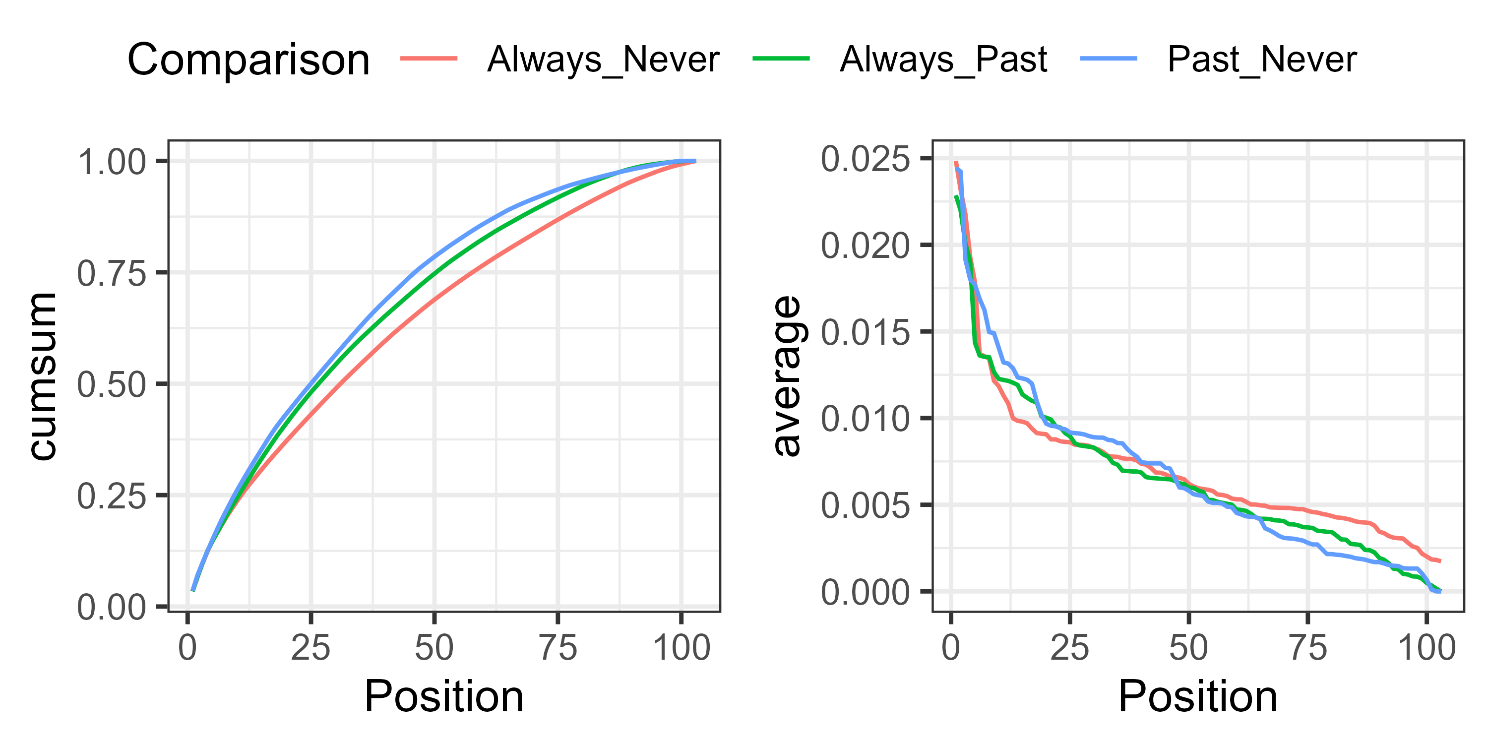
In this case, the cumulative contribution of species is more even for the Always_Never comparison than for the others (left), and every species contributes some non-zero amount to the compositional difference (right).

Code to create the above graphic follows:

p1 <- ggplot(data = simper.results,
aes(x = Position, y = cumsum)) +
geom_line(aes(colour = Comparison)) +
theme_bw()

p2 <- ggplot(data = simper.results,
aes(x = Position, y = average)) +
geom_line(aes(colour = Comparison)) +
theme_bw()

library(ggpubr)

ggarrange(p1, p2, common.legend = TRUE)

ggsave("graphics/simper.Grazing.png", width = 5, height = 2.5,
units = "in", dpi = 600)

Conclusions

The help files (?simper) provide some caveats for the interpretation of SIMPER.  For example:

"The method gives the contribution of each species to overall dissimilarities, but these are caused by variation in species abundances, and only partly by differences among groups. Even if you make groups that are copies of each other, the method will single out species with high contribution, but these are not contributions to non-existing between-group differences but to random noise variation in species abundances."

In general, this approach doesn’t appear to have received much attention from ecologists – perhaps because of these concerns about how to interpret the results - though the work of Gibert & Escarguel (2019) suggests that other ways to use this information could be developed.  A few years later, Vilmi et al. (2021) extended Gibert & Escarguel's 2019 work into a dispersal-niche continuum index (DNCI) that is based on SIMPER analysis.

Each pair of groups is considered separately in SIMPER, whereas Indicator Species Analysis allows you to compare multiple groups to one another.  The two techniques can be combined together by, for example, using ISA to identify species that are significant indicators of a group and then using SIMPER to quantify the contributions of those species to the average differences between the groups.

Other ways to use the information summarized in SIMPER could be developed.  For example, comparing patterns within groups to patterns between groups might be a fruitful way forward.  And, SIMPER analyses could be applied to presence/absence data.

References

Clarke, K.R. 1993. Non-parametric multivariate analyses of changes in community structure. Australian Journal of Ecology 18:117-143.

da Costa, P.B., S.B. de Campos, A. Albersmeier, P. Dirksen, A.L.P. Dresseno, O.J.A.P. dos Santos, K.M.L. Milani, R.M. Etto, A.G. Battistus, A.C.P.R. da Costa, A.L.M. de Oliveira, C.W. Galvão, V.F. Guimarães, A. Sczyrba, V.F. Wendisch, and L.M.P. Passaglia. 2018. Invasion ecology applied to inoculation of plant growth promoting bacteria through a novel SIMPER-PCA approach. Plant and Soil 422:467-478.

Encarnação, J., F. Leitão, P. Range, D. Piló, M.A. Chícharo, and L. Chícharo. 2015. Local and temporal variations in near-shore macrobenthic communities associated with submarine groundwater discharges. Marine Ecology 36(4):926-941.

Evangelista, A., L. Frate, M.L. Carranza, F. Attore, G. Pelino, and A. Stanisci. 2016. Changes in composition, ecology and structure of high-mountain vegetation: a re-visitation study over 42 years. AoB Plants 8:plw004.

Gibert, C., and G. Escarguel. 2019. PER-SIMPER—A new tool for inferring community assembly processes from taxon occurrences. Global Ecology and Biogeography 28(3):374-385.

Vilmi, A., C. Gibert, G. Escarguel, K. Happonen, J. Heino, A. Jamoneau, S.I. Passy, F. Picazo, J. Soininen, J. Tison-Rosebery, and J. Wang. 2021. Dispersal–niche continuum index: a new quantitative metric for assessing the relative importance of dispersal versus niche processes in community assembly. Ecography 44(3):370-379.

Yeager, M.E., and A.R. Hughes. 2025. Functional trait analysis reveals the hidden stability of multitrophic communities. Ecology 106(2):e70001.