
15 Demand, Supply, and Economic Efficiency
LEARNING OBJECTIVES
Type your learning objectives here.
- To differentiate between equity and efficiency, within an economic context
- To learn how economic surplus – the total of consumer and producer surplus – can be used to analyze questions of equity and efficiency
Equity deals with how society’s goods and rewards are, and should be, distributed among its different members, and how the associated costs should be apportioned.
Efficiency addresses the question of how well the economy’s resources are used and allocated.
Equity is also concerned with how different generations share an economy’s productive capabilities: More investment today makes for a more productive economy tomorrow, but more greenhouse gases today will reduce environmental quality tomorrow. These are inter-generational questions. Climate change caused by global warming forms one of the biggest challenges for humankind at the present time. As we shall see in this chapter, economics has much to say about appropriate policies to combat warming. Whether pollution-abatement policies should be implemented today or down the road involves considerations of equity between generations. Our first task is to develop an analytical tool which will prove vital in assessing and computing welfare benefits and costs – economic surplus.
Consumer and producer surplus
An understanding of economic efficiency is greatly facilitated as a result of understanding two related measures: Consumer surplus and producer surplus. Consumer surplus relates to the demand side of the market, producer surplus to the supply side. Producer surplus is also termed supplier surplus. These measures can be understood with the help of a standard example, the market for city apartments.
The market for apartments
Table 5.1 describes the hypothetical data. We imagine first a series of city-based students who are in the market for a standardized downtown apartment. These individuals are not identical; they value the apartment differently. For example, Alex enjoys comfort and therefore places a higher value on a unit than Brian. Brian, in turn, values it more highly than Cathy or Don.
Evan and Frank would prefer to spend their money on entertainment, and so on. These valuations are represented in the middle column of the demand panel in Table 5.1. The valuations reflect the willingness to pay of each consumer.
Demand
| Individual | Demand Valuation | Surplus |
| Alex | 900 | 400 |
| Brian | 800 | 300 |
| Cathy | 700 | 200 |
| Don | 600 | 100 |
| Eliza | 500 | 0 |
| Frank | 400 | 0 |
Supply
| Individual | Reservation Value | Surplus |
| Gladys | 300 | 200 |
| Howard | 350 | 150 |
| Ione | 400 | 100 |
| Jeff | 450 | 50 |
| Kirin | 500 | 0 |
| Lynn | 550 | 0 |
Table 2. – Demand Valuations and Supply Reservation Values
On the supply side we imagine the market as being made up of different individuals or owners, who are willing to put their apartments on the market for different prices. Gladys will accept less rent than Howard, who in turn will accept less than Ione. The minimum prices that the suppliers are willing to accept are called reservation prices or values, and these are given in the lower part of Table 5.1. Unless the market price is greater than their reservation price, suppliers will hold back. Likewise, the reservation values of the suppliers form the supply curve. If Alex is willing to pay $900, then that is her demand price; if Howard is willing to put his apartment on the market for $350, he is by definition willing to supply it for that price.
In this example, the equilibrium price for apartments will be $500. Let us see why. At that price the value placed on the marginal unit supplied by Kirin equals Eliza’s willingness to pay. Five apartments will be rented. A sixth apartment will not be rented because Lynn will rent her apartment only if the price reaches $550. But the sixth potential demander is willing to pay only $400. Note that, as usual, there is just a single price in the market. Each renter pays $500, and therefore each supplier also receives $500. The consumer and supplier surpluses can now be computed. Note that, while Don is willing to pay $600, he actually pays $500. His consumer surplus is therefore $100. These values are given in the final column of the top half of Table 5.1.
Consumer surplus is the excess of consumer willingness to pay over the market price.
Using the same reasoning, we can compute each supplier’s surplus, which is the excess of the amount obtained for the rented apartment over the reservation price. For example, Howard obtains a surplus on the supply side of $150, while Jeff gets $50. Howard is willing to put his apartment on the market for $350, but gets the equilibrium price/rent of $500 for it. Hence his surplus is $150.
Supplier or producer surplus is the excess of market price over the reservation price of the supplier.
It should now be clear why these measures are called surpluses. The suppliers and demanders are all willing to participate in this market because they earn this surplus. It is a measure of their gain from being involved in the trading. The sum of each participant’s surplus in the final column of Table 5.1 defines the total surplus in the market. Hence, on the demand side a total surplus arises of $1,000 and on the supply side a value of $500.
Another Example: The taxi market
Usually there are so many participants in the market that the differences in reservation prices on the supply side and willingness to pay on the demand side are exceedingly small, and so the demand and supply curves are drawn as continuous lines. So our second example reflects this, and comes from the market for taxi rides. We might think of this as an Uber- or Lyft-type taxi
operation. Let us suppose that the demand and supply curves for taxi rides in a given city are given by the functions in Figure 5.2.
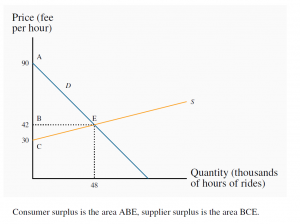
Figure 2. – Consumer surplus in the taxi market
The demand curve represents the willingness to pay on the part of riders. The supply curve represents the willingness to supply on the part of drivers. The price per hour of rides defines the vertical axis; hours of rides (in thousands) are measured on the horizontal axis. The demand intercept of $90 says that the person who values the ride most highly is willing to pay $90 per hour.
The downward slope of the demand curve states that other buyers are willing to pay less. On the supply side no driver is willing to supply his time and vehicle unless he obtains at least $30 per hour. To induce additional suppliers a higher price must be paid, and this is represented by the upward sloping supply curve.
The intersection occurs at a price of $42 per hour and the equilibrium number of ride-hours supplied is 48 thousand1. Computing the surpluses is very straightforward. By definition the consumer surplus is the excess of the willingness to pay by each buyer above the uniform price. Buyers who value the ride most highly obtain the biggest surplus – the highest valuation rider gets a surplus of $48 per hour – the difference between his willingness to pay of $90 and the actual price of $42. Each successive rider gets a slightly lower surplus until the final rider, who obtains zero. She pays $42 and values the ride hours at $42 also. On the supply side, the drivers who are willing to supply rides at the lowest reservation price ($30 and above) obtain the biggest surplus. The ‘marginal’ supplier gets no surplus, because the price equals her reservation price. From this discussion it follows that the consumer surplus is given by the area ABE and the supplier surplus by the area CBE. These are two triangular areas, and measured as half of the base by the perpendicular height. Therefore, in thousands of units:
Consumer Surplus = (demand value – price) = area ABE
= (1/2)×48×$48 = $1,152
Producer Surplus = (price – reservation supply value) = area BEC
= (1/2)×48×$12 = $288
The total surplus that arises in the market is the sum of producer and consumer surpluses, and since
the units are in thousands of hours the total surplus here is ($1,152+$288)×1,000=$1,440,000.
Efficient market outcomes
The definition and measurement of the surplus is straightforward provided the supply and demand functions are known. An important characteristic of the marketplace is that in certain circumstances it produces what we call an efficient outcome, or an efficient market. Such an outcome yields the highest possible sum of surpluses.
An efficient market maximizes the sum of producer and consumer surpluses.
