
18 Consumer Preferences
What it means for Consumers to be Rational
In order to analyze the choices that consumers make in a formal way, it is necessary for consumers to behave in a rational manner. The first assumption we will make about consumers is that they are able to compare any two options by saying that either they like one better than the other or that they are completely indifferent between the two. In other words, we assume that preferences are complete. Sometimes we are offered a choice between two undesirable alternatives. Does this imply that we have incomplete preferences? Absolutely not. If a vegetarian is offered a choice between ham and turkey, they will report that they are indifferent—they receive exactly zero satisfaction, or utility, from either option!
The second assumption we will make about consumers is that they have consistent preferences. If you report that you prefer tacos to sushi and that you prefer sushi to burgers, then it must be the case that you prefer tacos to sushi. The assumption we are making here is that preferences are transitive. Transitivity also works with indifference between two options: if you are indifferent between jogging and swimming and you prefer cycling to swimming, then you must also prefer cycling to jogging. While this assumption may seem uncontroversial for an individual consumer, transitivity may fail to hold if we aggregate the preferences of a group. It is possible that a group of friends could vote for tacos over sushi and sushi over burgers but then vote for burgers over tacos. In what follows, however, we will consider only the preferences of a single individual.
These rationality assumptions do not imply that everyone will make the same choices or that consumers always make the choice that turns out to be best for them. Risky decisions and poorly informed decisions can also be perfectly rational decisions. What our assumptions do mean is that consumers are capable of choosing among alternatives and that their rankings of those alternatives are logically consistent.
Another common, but somewhat more controversial assumption that economists make is that consumers believe that more is better. By qualifying this statement slightly, we can have more confidence that it will hold for consumers in general. First, more of an economic good is better. Other things being equal, more disease is clearly not better. Disease in this case would be considered an economic bad. We can still analyze consumers’ choices regarding disease by considering a related good rather than the bad itself: health would be a good and, other things equal, more health would be better. Other times, we consume so much of a good that it actually lowers our overall utility. You may love pizza, but it is possible to eat too much and end up feeling sick. In this case, more doesn’t turn out to be better. There are two reasons that this is at most a minor problem for our study of consumer choice. First, what we really mean is that a little more is better. Is one more bite of pizza better? The answer is probably yes. Second, even if one more bite of pizza makes us sick the important thing is that when we made the decision to take that bite we believed that one more was going to be better. In any case, it is a good idea to be aware of this assumption and realize when it might not hold so that we can adjust our analysis accordingly.
Based on the more is better assumption, we can already make one prediction about the choice that consumers will make. Consumers will choose a point on the budget line rather than the interior of the budget set. In other words, consumers will spend all of their income. Otherwise, they could afford more of either or both goods thereby making themselves better off. Keep in mind that this does not preclude savings. Future consumption can be considered a good just like any other and we can allocate some of our income to savings and still be considered to be spending all of our income.
Indifference Curves: A Graphical Representation of Preferences
Rather than trying to compare each and every combination of goods that a person can buy, we can use a graph to represent preferences among these combinations in a simple way. An indifference curve shows graphically all combinations of goods that provide an equal level of utility. In other words, an indifference curve shows all combinations of goods among which the consumer is indifferent. Indifference curves allow us to graphically depict the amount of utility a consumer derives from two goods and to rank all potential combinations of those goods. For example, Figure 4.10 shows three indifference curves that represent Lilly’s preferences for the tradeoffs that she faces in her two main relaxation activities: eating doughnuts and reading paperback books. Each indifference curve (UL, UM, and UH) represents one level of utility. First we will explore the meaning of one particular indifference curve and then we will look at the indifference curves as a group.
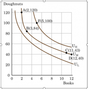
Figure 4.10 Indifference curves
Characteristics of Indifference Curves
The indifference curve UM has four points labeled on it: A, B, C, and D. Since an indifference curve represents a set of choices that have the same level of utility, Lilly must receive an equal amount of utility, judged according to her personal preferences, from two books and 120 doughnuts (point A), from three books and 84 doughnuts (point B) from 11 books and 43 doughnuts (point C) or from 12 books and 40 doughnuts (point D). She would also receive the same utility from any of the unlabeled intermediate points along this indifference curve.
The assumptions we have made about preferences tell us quite a bit about how indifference curves should look. For example, we know that Lilly’s indifference curves will be negatively sloped because of our assumption that more is better. If we give her more books, we will have to take away some doughnuts or else she will be made better off. Likewise, we would need to take away some books in order to keep her indifferent if we were to give her more doughnuts.
In addition to being downward sloping from left to right, indifference curves tend to be convex with respect to the origin. In other words, they are steeper on the left and flatter on the right. The slope of an indifference curve tells us how much of the good on the vertical axis (doughnuts in Lilly’s case) the consumer is willing to give up in order to consume one additional unit of the good on the horizontal axis (books for Lilly). Contrast this with the slope of the consumer’s budget line, which tells us how much of the good on the vertical axis
must be given up in exchange for one additional unit of the good on the horizontal axis. This willingness to trade one good for a marginal (i.e., one unit) increase in the other good while holding total utility constant is known as the Marginal Rate of Substitution (MRS).
The convex shape of typical indifference curves means that the marginal rate of substitution decreases as we move down along an indifference curve. This shape results from another of our assumptions: that the law of diminishing marginal utility holds. Thus, the increase in utility that Lilly would gain from, say, increasing her consumption of books from two to three must be equal to the decrease in utility when her consumption of doughnuts was cut from 120 to 84 so that her overall utility remains unchanged between points A and B. At
point A, where she has relatively large number of doughnuts and therefore her marginal utility from doughnuts will be relatively small. At the same time, she has relatively few books and therefore has a relatively high marginal utility for books. Viewed in terms of the marginal utilities of the two goods, it is easy to see why Lilly is willing to give up 36 doughnuts to increase the number of books she has from 2 to 3. When Lilly has a larger
number of books and fewer doughnuts at point C in Figure 4, she will have a lower marginal utility for books and a higher marginal utility for doughnuts. In going from point C to point D, she is only willing to give up 3 of the now precious doughnuts for yet another book.
Computationally, the MRS is equal to the ratio of the marginal utilities of the two goods:
[latex][/latex] MRS_Y,X = \frac{MU_X}}{MU_Y}
To understand why this is true, consider a consumer who receives MUX = 20 from good X and MUY = 4 from good Y. How many units of good Y would the consumer be willing to substitute for one additional unit of good X? The one additional unit of good X will increase her total utility by 20. To remain on the same indifference curve, we need a decrease in good Y that will exactly offset this increase. A decrease of 5 units of good Y, which each give her 4 units of utility, known as utils, at the margin will lower total utility by the necessary 20 utils, leaving Lilly’s overall utility unchanged:
[latex][/latex] MRS_Y,X = \frac{20}{4} = 5
Our assumption that preferences are complete implies that there exists an indifference curve through every combination. Thus, Lilly’s preferences will include an infinite number of indifference curves lying nestled together on the diagram—even though only three of the indifference curves, representing three levels of utility, appear on Figure 4. In other words, an infinite number of indifference curves are not drawn on this diagram but you should remember that they exist.
The combination of the more is better and transitivity assumptions assure us that higher indifference curves represent a greater level of utility than lower ones. In Figure 4, indifference curve UL can be thought of as a “low” level of utility, while UM is a “medium” level of utility and UH is a “high” level of utility. All of the choices on indifference curve UH are preferred to all of the choices on indifference curve UM, which in turn are preferred to all of the choices on UL.
To understand why higher indifference curves are preferred to lower ones, compare point B on indifference curve UM to point F on indifference curve UH. Point F has greater consumption of both books (5 to 3) and doughnuts (100 to 84), so point F is clearly preferable to point B due to our assumption that more is better. The more is better assumption, however, does not allow us to directly compare point F to point C, since point F has more has more doughnuts but point C has more books. Transitivity gives us the desired result: since point F is preferable to point B and point B gives the same level of utility as point C, point F is also preferable to point C. Given the definition of an indifference curve—that all the points on the curve have the same level of utility—if point F on indifference curve UH is preferred to point B on indifference curve UM, then it must be true that all points on indifference curve UH have a higher level of utility than all points on UM.
More generally, for any point on a lower indifference curve, like UL, you can identify a point on a higher indifference curve like UM or UH that has a higher consumption of both goods. Since one point on the higher indifference curve is preferred to one point on the lower curve, and since all the points on a given indifference curve have the same level of utility, it must be true that all points on higher indifference curves have greater utility than all points on lower indifference curves. A final point to note is that indifference curves never cross. If they did, then we would have a single combination—where the curves intersect—that would be assigned two levels of utility and transitivity would be violated.
These arguments about the shapes of indifference curves and about higher or lower levels of utility do not require any numerical estimates of utility, either by the individual or by anyone else. They are only based on the assumptions that we have made in this section. Given these gentle assumptions, an indifference map can be constructed to describe the preferences of any individual.
The Individuality of Indifference Curves and Special Cases
Each person determines their own preferences and utility. Thus, while indifference curves have the same general characteristics—they exist, they are downward sloping, and they never cross—the specific shape of indifference curves can be different for every person. Figure 4, for example, applies only to Lilly’s preferences. Indifference curves for other people would probably travel through different points. Also, the convexity of typical indifference curves is just that—typical. Not all indifference curves have this same type of curvature. Figure 5 shows two examples of indifference curves that are not convex to the origin.
In Figure 5-a we have Jim’s preferences over left shoes and right shoes. These goods are perfect complements for Jim, meaning he always consumes them together. The bend in the indifference curves represents situations where Jim has equal amounts of left and right shoes, meaning he has a number of complete pairs of shoes. If, starting from Point A where Jim has exactly five pairs of shoes, we were to give him an extra right shoe would he be made better off? Not likely. Point B, where Jim has five left shoes and six right shoes, is therefore on the same indifference curve as Point A. The same would be true if we were to increase only his consumption of right shoes. Indifference curves for perfect complements are therefore L-shaped. Notice that not all examples of perfect complements are consumed in a 1:1 ratio. If you wear glasses, for example, you likely consume two lenses for each set of frames. Since perfect complements are always consumed together in a constant ratio, it is unsurprising that they also tend to be sold together as a bundle.
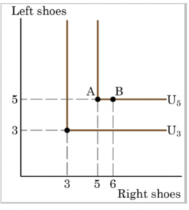
Figure 4.11 Perfect Complements
Figure 5-b shows Sally’s preferences for blue pencils and yellow pencils. Since Sally has no preference over the color of the pencil she uses, the goods are perfect substitutes. She will trade one blue pencil for an additional yellow pencil no matter how many of each she has currently. What matters to Sally is not the number of each color but the total number of pencils. In this case the marginal rate of substitution is constant which implies that the indifference curves are linear. The key to perfect substitutes is that the marginal rate of substitution is constant, not that it is necessarily equal to one. Sally would be willing to trade 2 five-packs of pencils for one 1 ten-pack of pencils regardless of how many of each size package she has currently.
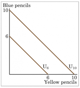
Figure 4.12 Perfect Substitutes
