Multiple Linear Regression

Barbara Illowsky; Margo Bergman; Susan Dean

13 Multiple Linear Regression

Barbara Illowsky; Margo Bergman; and Susan Dean

Student Learning Outcomes

By the end of this chapter, the student should be able to:

Perform and interpret multiple regression analysis
State the assumptions of OLS regression and why they are important
Discusses the causes and corrections of multicollinearity
Explain the purpose and method of including dummy variables
Explain the purpose and method of logarithmic transformations
Develop predictions of data with multiple regression equations

The Multiple Linear Regression Equation

As previously stated, regression analysis is a statistical technique that can test the hypothesis that a variable is dependent upon one or more other variables. Further, regression analysis can provide an estimate of the magnitude of the impact of a change in one variable on another. This last feature, of course, is all important in predicting future values.

Regression analysis is based upon a functional relationship among variables and further, assumes that the relationship is linear. This linearity assumption is required because, for the most part, the theoretical statistical properties of non-linear estimation are not well worked out yet by the mathematicians and econometricians. This presents us with some difficulties in economic analysis because many of our theoretical models are nonlinear. The marginal cost curve, for example, is decidedly nonlinear as is the total cost function, if we are to believe in the effect of specialization of labor and the Law of Diminishing Marginal Product. There are techniques for overcoming some of these difficulties, exponential and logarithmic transformation of the data for example, but at the outset we must recognize that standard ordinary least squares (OLS) regression analysis will always use a linear function to estimate what might be a nonlinear relationship. When there is only one independent, or explanatory variable, we call the relationship simple linear regression. When there is more than one independent variable, we refer to performing multiple linear regression.

The general multiple linear regression model can be stated by the equation:

$y_i=\beta_0+\beta_1X_{1i}+\beta_2X_{2i}+...+\beta_kX_{ki}+\epsilon_i$

where $\beta_0$ is the intercept, $\beta_i$ ‘s are the slope between Y and the appropriate $X_i$ , and $\epsilon$ (pronounced epsilon), is the error term that captures errors in measurement of Y and the effect on Y of any variables missing from the equation that would contribute to explaining variations in Y. This equation is the theoretical population equation and therefore uses Greek letters. The equation we will estimate will have the Roman equivalent symbols. This is parallel to how we kept track of the population parameters and sample parameters before. The symbol for the population mean was $\mu$ and for the sample mean $\bar{x}$ and for the population standard deviation was $\sigma$ and for the sample standard deviation was s. The equation that will be estimated with a sample of data for two independent variables will thus be:

$y_i=b_0+b_1x_{1i}+b_2x_{2i}+e_i$

As with all probability distributions, this model works only if certain assumptions hold. These are that the Y is normally distributed, the errors are also normally distributed with a mean of zero and a constant standard deviation, and that the error terms are independent of the size of X and independent of each other.

Assumptions of the Ordinary Least Squares Regression Model

Each of these assumptions needs a bit more explanation. If one of these assumptions fails to be true, then it will have an effect on the quality of the estimates. Some of the failures of these assumptions can be fixed while others result in estimates that quite simply provide no insight into the questions the model is trying to answer or worse, give biased estimates.

The independent variables, $x_i$ , are all measured without error, and are fixed numbers that are independent of the error term. This assumption is saying in effect that Y is deterministic, the result of a fixed component “X” and a random error component “ $\epsilon$ ”.
The error term is a random variable with a mean of zero and a constant variance. The meaning of this is that the variances of the independent variables are independent of the value of the variable. Consider the relationship between personal income and the quantity of a good purchased as an example of a case where the variance is dependent upon the value of the independent variable, income. It is plausible that as income increases the variation around the amount purchased will also increase simply because of the flexibility provided with higher levels of income. The assumption is for constant variance with respect to the magnitude of the independent variable called homoscedasticity. If the assumption fails, then it is called heteroscedasticity. Figure 1 shows the case of homoscedasticity where all three distributions have the same variance around the predicted value of Y regardless of the magnitude of X.
While the independent variables are all fixed values they are from a probability distribution that is normally distributed. This can be seen in Figure 1 by the shape of the distributions placed on the predicted line at the expected value of the relevant value of Y.
The independent variables are independent of Y, but are also assumed to be independent of the other X variables. The model is designed to estimate the effects of independent variables on some dependent variable in accordance with a proposed theory. The case where some or more of the independent variables are correlated is not unusual. There may be no cause and effect relationship among the independent variables, but nevertheless they move together. Take the case of a simple supply curve where quantity supplied is theoretically related to the price of the product and the prices of inputs. There may be multiple inputs that may over time move together from general inflationary pressure. The input prices will therefore violate this assumption of regression analysis. This condition is called multicollinearity, which will be taken up in detail later.
The error terms are uncorrelated with each other. This situation arises from an effect on one error term from another error term. While not exclusively a time series problem, it is here that we most often see this case. An X variable in time period one has an effect on the Y variable, but this effect then has an effect in the next time period. This effect gives rise to a relationship among the error terms. This case is called autocorrelation, “self-correlated.” The error terms are now not independent of each other, but rather have their own effect on subsequent error terms.

Figure 1 shows the case where the assumptions of the regression model are being satisfied. The estimated line is $\^y=b+mx$ . Three values of X are shown. A normal distribution is placed at each point where X equals the estimated line and the associated error at each value of Y. Notice that the three distributions are normally distributed around the point on the line, and further, the variation, variance, around the predicted value is constant indicating homoscedasticity from assumption 2. Figure 1 does not show all the assumptions of the regression model, but it helps visualize these important ones.

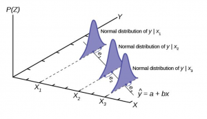
Figure 1

Multicollinearity

Our discussion earlier indicated that like all statistical models, the OLS regression model has important assumptions attached. Each assumption, if violated, has an effect on the ability of the model to provide useful and meaningful estimates. The Gauss-Markov Theorem has assured us that the OLS estimates are unbiased and minimum variance, but this is true only under the assumptions of the model. Here we will look at the effects on OLS estimates if the independent variables are correlated. The other assumptions and the methods to mitigate the difficulties they pose if they are found to be violated are examined in Econometrics courses. We take up multicollinearity because it is so often prevalent in Economic models and it often leads to frustrating results.

The OLS model assumes that all the independent variables are independent of each other. This assumption is easy to test for a particular sample of data with simple correlation coefficients. Correlation, like much in statistics, is a matter of degree: a little is not good, and a lot is terrible.

The goal of the regression technique is to tease out the independent impacts of each of a set of independent variables on some hypothesized dependent variable. If two 2 independent variables are interrelated, that is, correlated, then we cannot isolate the effects on Y of one from the other. In an extreme case where $x_1$ ‘s a linear combination of $x_2$ , correlation equal to one, both variables move in identical ways with Y. In this case it is impossible to determine the variable that is the true cause of the effect on Y. (If the two variables were actually perfectly correlated, then mathematically no regression results could actually be calculated.)

The correlation between $x_1$ and $x_2$ , $r{^2}_{x_1x_2}$ appears in the denominator of both the estimating formula for $b_1$ and $b_2$ . If the assumption of independence holds, then this term is zero. This indicates that there is no effect of the correlation on the coefficient. On the other hand, as the correlation between the two independent variables increases the denominator decreases, and thus the estimate of the coefficient increases. The correlation has the same effect on both of the coefficients of these two variables. In essence, each variable is “taking” part of the effect on Y that should be attributed to the collinear variable. This results in biased estimates.

Multicollinearity has a further deleterious impact on the OLS estimates. The correlation between the two independent variables also shows up in the formulas for the estimate of the variance for the coefficients. If the correlation is zero as assumed in the regression model, then the formula collapses to the familiar ratio of the variance of the errors to the variance of the relevant independent variable. If however the two independent variables are correlated, then the variance of the estimate of the coefficient increases. This results in a smaller t-value for the test of hypothesis of the coefficient. In short, multicollinearity results in failing to reject the null hypothesis that the X variable has no impact on Y when in fact X does have a statistically significant impact on Y. Said another way, the large standard errors of the estimated coefficient created by multicollinearity suggest statistical insignificance even when the hypothesized relationship is strong.

Dummy Variables

Thus far the analysis of the OLS regression technique assumed that the independent variables in the models tested were continuous random variables. There are, however, no restrictions in the regression model against independent variables that are binary. This opens the regression model for testing hypotheses concerning categorical variables such as gender, race, region of the country, before a certain data, after a certain date and innumerable others. These categorical variables take on only two values, 1 and 0, success or failure, from the binomial probability distribution. The form of the equation becomes:

$\^y = b_0+b_2X_2+b_1X_1$

where $X_2$ = 0, 1 . $X_2$ is the dummy variable and $X_1$ is some continuous random variable. The constant, $b_0$ , is the y-intercept, the value where the line crosses the y-axis. When the value of $X_2$ = 0, the estimated line crosses at $b_0$ . When the value of $X_2$ = 1 then the estimated line crosses at $b_0 + b_2$ . In effect the dummy variable causes the estimated line to shift either up or down by the size of the effect of the characteristic captured by the dummy variable. Note that this is a simple parallel shift and does not affect the impact of the other independent variable; $X_1$ . This variable is a continuous random variable and predicts different values of y at different values of $X_1$ holding constant the condition of the dummy variable (Figure 2).

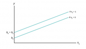
Figure 2

An example of the use of a dummy variable is the work estimating the impact of gender on salaries. There is a full body of literature on this topic and dummy variables are used extensively. For this example the salaries of elementary and secondary school teachers for a particular state is examined. Using a homogeneous job category, school teachers, and for a single state reduces many of the variations that naturally effect salaries such as differential physical risk, cost of living in a particular state, and other working conditions. The estimating equation in its simplest form specifies salary as a function of various teacher characteristic that economic theory would suggest could affect salary. These would include education level as a measure of potential productivity, age and/or experience to capture on-the-job training, again as a measure of productivity. Because the data are for school teachers employed in a public school districts rather than workers in a for-profit company, the school district’s average revenue per average daily student attendance is included as a measure of ability to pay. The results of the regression analysis using data on 24,916 school teachers are presented below.

Variable	Regression Coefficients (b)	Standard Errors of the Estimates for Teacher’s Earnings Function (sb)
Intercept	4269.9
Gender (male = 1)	632.38	13.39
Total Years of Experience	52.32	1.10
Years of Experience in Current District	29.97	1.52
Education	629.33	13.16
Total Revenue per ADA	90.24	3.76
R– 2	.725
n	24,916

Table 1: Earnings Estimate for Elementary and Secondary School Teachers

The coefficients for all the independent variables are significantly different from zero as indicated by the standard errors. Dividing the standard errors of each coefficient results in a t-value greater than 1.96 which is the required level for 95% significance. The binary variable, our dummy variable of interest in this analysis, is gender where male is given a value of 1 and female given a value of 0. The coefficient is significantly different from zero with a dramatic t-statistic of 47 standard deviations. We thus cannot accept the null hypothesis that the coefficient is equal to zero. Therefore we conclude that there is a premium paid male teachers of $632 after holding constant experience, education and the wealth of the school district in which the teacher is employed. It is important to note that these data are from some time ago and the $632 represents a six percent salary premium at that time. A graph of this example of dummy variables is presented below (Figure 3).

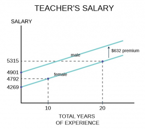
Figure 3

In two dimensions, salary is the dependent variable on the vertical axis and total years of experience was chosen for the continuous independent variable on horizontal axis. Any of the other independent variables could have been chosen to illustrate the effect of the dummy variable. The relationship between total years of experience has a slope of $52.32 per year of experience and the estimated line has an intercept of $4,269 if the gender variable is equal to zero, for female. If the gender variable is equal to 1, for male, the coefficient for the gender variable is added to the intercept and thus the relationship between total years of experience and salary is shifted upward parallel as indicated on the graph. Also marked on the graph are various points for reference. A female school teacher with 10 years of experience receives a salary of $4,792 on the basis of her experience only, but this is still $109 less than a male teacher with zero years of experience.

A more complex interaction between a dummy variable and the dependent variable can also be estimated. It may be that the dummy variable has more than a simple shift effect on the dependent variable, but also interacts with one or more of the other continuous independent variables. While not tested in the example above, it could be hypothesized that the impact of gender on salary was not a one-time shift, but impacted the value of additional years of experience on salary also. That is, female school teacher’s salaries were discounted at the start, and further did not grow at the same rate from the effect of experience as for male school teachers. This would show up as a different slope for the relationship between total years of experience for males than for females. If this is so then females school teachers would not just start behind their male colleagues (as measured by the shift in the estimated regression line), but would fall further and further behind as time and experienced increased.

The graph below shows how this hypothesis can be tested with the use of dummy variables and an interaction variable (Figure 4).

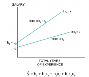
Figure 4

The estimating equation shows how the slope of $X_1$ , the continuous random variable experience, contains two parts, $b_1$ and $b_3$ . This occurs because of the new variable $X_2X_1$ , called the interaction variable, was created to allow for an effect on the slope of $X_1$ from changes in $X_2$ , the binary dummy variable. Note that when the dummy variable, $X_2$ = 0 the interaction variable has a value of 0, but when $X_2$ = 1 the interaction variable has a value of $X_1$ . The coefficient $b_3$ is an estimate of the difference in the coefficient of $X_1$ when $X_2$ = 1 compared to when $X_2$ = 0. In the example of teacher’s salaries, if there is a premium paid to male teachers that affects the rate of increase in salaries from experience, then the rate at which male teachers’ salaries rises would be $b_1 + b_3$ and the rate at which female teachers’ salaries rise would be simply $b_1$ . This hypothesis can be tested with the hypothesis:

$H_0:\beta_3=0|\beta_1=0,\beta_2=0$

$H_a:\beta_3=0|\beta_1\neq0,\beta_2\neq0$

This is a t-test using the test statistic for the parameter $\beta_3$ . If we cannot accept the null hypothesis that $\beta_3=0$ we conclude there is a difference between the rate of increase for the group for whom the value of the binary variable is set to 1, males in this example. This estimating equation can be combined with our earlier one that tested only a parallel shift in the estimated line. The earnings/experience functions in Figure 4 are drawn for this case with a shift in the earnings function and a difference in the slope of the function with respect to total years of experience.

Interpretation of Regression Coefficients: Elasticity and Logarithmic Transformation

Elasticity

As we have seen, the coefficient of an equation estimated using OLS regression analysis provides an estimate of the slope of a straight line that is assumed be the relationship between the dependent variable and at least one independent variable. From the calculus, the slope of the line is the first derivative and tells us the magnitude of the impact of a one unit change in the X variable upon the value of the Y variable measured in the units of the Y variable. As we saw in the case of dummy variables, this can show up as a parallel shift in the estimated line or even a change in the slope of the line through an interactive variable. Here we wish to explore the concept of elasticity and how we can use a regression analysis to estimate the various elasticities in which economists have an interest.

The concept of elasticity is borrowed from engineering and physics where it is used to measure a material’s responsiveness to a force, typically a physical force such as a stretching/pulling force. It is from here that we get the term an “elastic” band. In economics, the force in question is some market force such as a change in price or income. Elasticity is measured as a percentage change/response in both engineering applications and in economics. The value of measuring in percentage terms is that the units of measurement do not play a role in the value of the measurement and thus allows direct comparison between elasticities. As an example, if the price of gasoline increased say 50 cents from an initial price of $3.00 and generated a decline in monthly consumption for a consumer from 50 gallons to 48 gallons we calculate the elasticity to be 0.25. The price elasticity is the percentage change in quantity resulting from some percentage change in price. A 16 percent increase in price has generated only a 4 percent decrease in demand: 16% price change → 4% quantity change or .04/.16 = .25. This is called an inelastic demand meaning a small response to the price change. This comes about because there are few if any real substitutes for gasoline; perhaps public transportation, a bicycle or walking. Technically, of course, the percentage change in demand from a price increase is a decline in demand thus price elasticity is a negative number. The common convention, however, is to talk about elasticity as the absolute value of the number. Some goods have many substitutes: pears for apples for plums, for grapes, etc. etc. The elasticity for such goods is larger than one and are called elastic in demand. Here a small percentage change in price will induce a large percentage change in quantity demanded. The consumer will easily shift the demand to the close substitute.

While this discussion has been about price changes, any of the independent variables in a demand equation will have an associated elasticity. Thus, there is an income elasticity that measures the sensitivity of demand to changes in income: not much for the demand for food, but very sensitive for yachts. If the demand equation contains a term for substitute goods, say candy bars in a demand equation for cookies, then the responsiveness of demand for cookies from changes in prices of candy bars can be measured. This is called the cross-price elasticity of demand and to an extent can be thought of as brand loyalty from a marketing view. How responsive is the demand for Coca-Cola to changes in the price of Pepsi?

Now imagine the demand for a product that is very expensive. Again, the measure of elasticity is in percentage terms thus the elasticity can be directly compared to that for gasoline: an elasticity of 0.25 for gasoline conveys the same information as an elasticity of 0.25 for $25,000 car. Both goods are considered by the consumer to have few substitutes and thus have inelastic demand curves, elasticities less than one.

The mathematical formulae for various elasticities are:

Price elasticity: $\eta_p=\frac{\% \Delta Q}{\% \Delta P}$

where $\eta$ is the Greek small case letter eta used to designate elasticity. $\Delta$ is read as “change”.

Income elasticity: $\eta_Y=\frac{\% \Delta Q}{\% \Delta Y}$

Where Y is used as the symbol for income.

Cross-Price elasticity: $\eta_p1=\frac{\% \Delta Q_1}{\% \Delta P_2}$

Where P2 is the price of the substitute good.

Examining closer the price elasticity we can write the formula as:

$\eta_p=\frac{\% \Delta Q}{\% \Delta P}=\frac{dQ}{dP}\left(\frac{P}{Q}\right)=b\left(\frac{P}{Q}\right)$

Where b is the estimated coefficient for price in the OLS regression.

The first form of the equation demonstrates the principle that elasticities are measured in percentage terms. Of course, the ordinary least squares coefficients provide an estimate of the impact of a unit change in the independent variable, X, on the dependent variable measured in units of Y. These coefficients are not elasticities, however, and are shown in the second way of writing the formula for elasticity as $\frac{dQ}{dP}$ , the derivative of the estimated demand function which is simply the slope of the regression line. Multiplying the slope times $\frac{P}{Q}$ provides an elasticity measured in percentage terms.

Along a straight-line demand curve the percentage change, thus elasticity, changes continuously as the scale changes, while the slope, the estimated regression coefficient, remains constant. Going back to the demand for gasoline. A change in price from $3.00 to $3.50 was a 16 percent increase in price. If the beginning price were $5.00 then the same 50¢ increase would be only a 10 percent increase generating a different elasticity. Every straight-line demand curve has a range of elasticities starting at the top left, high prices, with large elasticity numbers, elastic demand, and decreasing as one goes down the demand curve, inelastic demand.

In order to provide a meaningful estimate of the elasticity of demand the convention is to estimate the elasticity at the point of means. Remember that all OLS regression lines will go through the point of means. At this point is the greatest weight of the data used to estimate the coefficient. The formula to estimate an elasticity when an OLS demand curve has been estimated becomes:

$\eta_p=b\left(\frac{\bar{P}}{\bar{Q}}\right)$

Where $\bar{P}$ and $\bar{Q}$ are the mean values of these data used to estimate b , the price coefficient.

The same method can be used to estimate the other elasticities for the demand function by using the appropriate mean values of the other variables; income and price of substitute goods for example.

Logarithmic Transformation of the Data

Ordinary least squares estimates typically assume that the population relationship among the variables is linear thus of the form presented in The Regression Equation. In this form the interpretation of the coefficients is as discussed above; quite simply the coefficient provides an estimate of the impact of a one unit change in X on Y measured in units of Y. It does not matter just where along the line one wishes to make the measurement because it is a straight line with a constant slope thus constant estimated level of impact per unit change. It may be, however, that the analyst wishes to estimate not the simple unit measured impact on the Y variable, but the magnitude of the percentage impact on Y of a one unit change in the X variable. Such a case might be how a unit change in experience, say one year, effects not the absolute amount of a worker’s wage, but the percentage impact on the worker’s wage. Alternatively, it may be that the question asked is the unit measured impact on Y of a specific percentage increase in X. An example may be “by how many dollars will sales increase if the firm spends X percent more on advertising?” The third possibility is the case of elasticity discussed above. Here we are interested in the percentage impact on quantity demanded for a given percentage change in price, or income or perhaps the price of a substitute good. All three of these cases can be estimated by transforming the data to logarithms before running the regression. The resulting coefficients will then provide a percentage change measurement of the relevant variable.

To summarize, there are four cases:

Unit $\Delta$ X → Unit $\Delta$ Y (Standard OLS case)
Unit $\Delta$ X → % $\Delta$ Y
% $\Delta$ X → Unit $\Delta$ Y
% $\Delta$ X → % $\Delta$ Y (elasticity case)

Case 1: The ordinary least squares case begins with the linear model developed above:

$Y=b_0+b_1x$

where the coefficient of the independent variable $b_1= \frac{dY}{dX}$ is the slope of a straight line and thus measures the impact of a unit change in X on Y measured in units of Y.

Case 2: The underlying estimated equation is:

$log Y=b_0+b_1X$

The equation is estimated by converting the Y values to logarithms and using OLS techniques to estimate the coefficient of the X variable, $b_1$ . This is called a semi-log estimation. Again, differentiating both sides of the equation allows us to develop the interpretation of the X coefficient $b_1$ :

$d log_Y = b_1 dX$

$\frac{dY}{Y} = {b_1}{dX}$

Multiply by 100 to covert to percentages and rearranging terms gives:

$100b_1 = \% \frac{\Delta Y}{\Delta X}$

$100b_1$ is thus the percentage change in Y resulting from a unit change in X.

Case 3: In this case the question is “what is the unit change in Y resulting from a percentage change in X?” What is the dollar loss in revenues of a five percent increase in price or what is the total dollar cost impact of a five percent increase in labor costs? The estimated equation for this case would be:

$Y=b_0+b_1 log (X)$

Here the calculus differential of the estimated equation is:

$dY=b_1d(logX)$

$dY=b_1\frac{dX}{X}$

Divide by 100 to get percentage and rearranging terms gives:

$\frac{b_1}{100}=\frac{dY}{100\frac{dX}{X}}=\frac{Unit \Delta Y}{\% \Delta X}$

Therefore, $\frac{b_1}{100}$ is the increase in Y measured in units from a one percent increase in X.

Case 4: This is the elasticity case where both the dependent and independent variables are converted to logs before the OLS estimation. This is known as the log-log case or double log case, and provides us with direct estimates of the elasticities of the independent variables. The estimated equation is:

$log Y=b_0+b_1 log (X)$

Differentiating we have:

$d (log Y)=b_1 d(logX)$

$d (log Y)=b_1\frac{1}{X}$

thus

$\frac{1}{Y} dY = b_1\frac{1}{X} \; OR \; \frac{dY}{Y} = b_1\frac{1}{X} \; OR \; b_1 =\frac{dY}{dX}\left(\frac{X}{Y}\right)$

and $b_1 =\frac{ \% \Delta Y}{ \% \Delta X}$

our definition of elasticity. We conclude that we can directly estimate the elasticity of a variable through double log transformation of the data. The estimated coefficient is the elasticity. It is common to use double log transformation of all variables in the estimation of demand functions to get estimates of all the various elasticities of the demand curve.

Predicting with a Multiple Regression Equation

One important value of an estimated regression equation is its ability to predict the effects on Y of a change in one or more values of the independent variables. The value of this is obvious. Careful policy cannot be made without estimates of the effects that may result. Indeed, it is the desire for particular results that drive the formation of most policy. Regression models can be, and have been, invaluable aids in forming such policies.

The Gauss-Markov theorem assures us that the point estimate of the impact on the dependent variable derived by putting in the equation the hypothetical values of the independent variables one wishes to simulate will result in an estimate of the dependent variable which is minimum variance and unbiased. That is to say that from this equation comes the best unbiased point estimate of y given the values of x.

$\^y=\b_0+\b_1X_{1i}+\b_2X_{2i}+...+\b_kX_{ki}$

Remember that point estimates do not carry a particular level of probability, or level of confidence, because points have no “width” above which there is an area to measure. This was why we developed confidence intervals for the mean and proportion earlier. The same concern arises here also. There are actually two different approaches to the issue of developing estimates of changes in the independent variable, or variables, on the dependent variable. The first approach wishes to measure the expected mean value of y from a specific change in the value of x: this specific value implies the expected value. Here the question is: what is the mean impact on y that would result from multiple hypothetical experiments on y at this specific value of x. Remember that there is a variance around the estimated parameter of x and thus each experiment will result in a bit of a different estimate of the predicted value of y.

The second approach to estimate the effect of a specific value of x on y treats the event as a single experiment: you choose x and multiply it times the coefficient and that provides a single estimate of y. Because this approach acts as if there were a single experiment the variance that exists in the parameter estimate is larger than the variance associated with the expected value approach.

The conclusion is that we have two different ways to predict the effect of values of the independent variable(s) on the dependent variable and thus we have two different intervals. Both are correct answers to the question being asked, but there are two different questions. To avoid confusion, the first case where we are asking for the expected value of the mean of the estimated y, is called a confidence interval as we have named this concept before. The second case, where we are asking for the estimate of the impact on the dependent variable y of a single experiment using a value of x, is called the prediction interval. The test statistics for these two interval measures within which the estimated value of y will fall are:

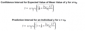
Where $s_e$ is the standard deviation of the error term and $s_x$ is the standard deviation of the x variable.

The mathematical computations of these two test statistics are complex. Various computer regression software packages provide programs within the regression functions to provide answers to inquires of estimated predicted values of y given various values chosen for the x variable(s). It is important to know just which interval is being tested in the computer package because the difference in the size of the standard deviations will change the size of the interval estimated. This is shown in Figure 5.

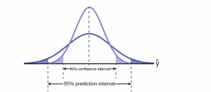
Figure 5

Figure 5 shows visually the difference the standard deviation makes in the size of the estimated intervals. The confidence interval, measuring the expected value of the dependent variable, is smaller than the prediction interval for the same level of confidence. The expected value method assumes that the experiment is conducted multiple times rather than just once as in the other method. The logic here is similar, although not identical, to that discussed when developing the relationship between the sample size and the confidence interval using the Central Limit Theorem. There, as the number of experiments increased, the distribution narrowed and the confidence interval became tighter around the expected value of the mean.

It is also important to note that the intervals around a point estimate are highly dependent upon the range of data used to estimate the equation regardless of which approach is being used for prediction. Remember that all regression equations go through the point of means, that is, the mean value of y and the mean values of all independent variables in the equation. As the value of x chosen to estimate the associated value of y is further from the point of means the width of the estimated interval around the point estimate increases. Choosing values of x beyond the range of the data used to estimate the equation possess even greater danger of creating estimates with little use; very large intervals, and risk of error. Figure 6 shows this relationship.

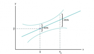
Figure 6

Figure 6 demonstrates the concern for the quality of the estimated interval whether it is a prediction interval or a confidence interval. As the value chosen to predict y, $X_p$ in the graph, is further from the central weight of the data, $\bar{X}$ , we see the interval expand in width even while holding constant the level of confidence. This shows that the precision of any estimate will diminish as one tries to predict beyond the largest weight of the data and most certainly will degrade rapidly for predictions beyond the range of the data. Unfortunately, this is just where most predictions are desired. They can be made, but the width of the confidence interval may be so large as to render the prediction useless. Only actual calculation and the particular application can determine this, however.

Third exam/final exam example

We found the equation of the best-fit line for the final exam grade as a function of the grade on the third-exam. We can now use the least-squares regression line for prediction. Assume the coefficient for X was determined to be significantly different from zero.

Suppose you want to estimate, or predict, the mean final exam score of statistics students who received 73 on the third exam. The exam scores (x-values) range from 65 to 75. Since 73 is between the x-values 65 and 75, we feel comfortable to substitute x = 73 into the equation. Then:

$\^y=− 173.51 + 4.83(73) = 179.08$

We predict that statistics students who earn a grade of 73 on the third exam will earn a grade of 179.08 on the final exam, on average.

What would you predict the final exam score to be for a student who scored a 66 on the third exam?

Solution – 1

145.27

2. What would you predict the final exam score to be for a student who scored a 90 on the third exam?

Solution – 2

The x values in the data are between 65 and 75. Ninety is outside of the domain of the observed x values in the data (independent variable), so you cannot reliably predict the final exam score for this student. (Even though it is possible to enter 90 into the equation for x and calculate a corresponding y value, the y value that you get will have a confidence interval that may not be meaningful.)

To understand really how unreliable the prediction can be outside of the observed x values observed in the data, make the substitution x = 90 into the equation.

$\^y=− 173.51 + 4.83(73) = 261.19$

The final-exam score is predicted to be 261.19. The largest the final-exam score can be is 200.

Media Attributions

RegAssumGraph
DummyGraph
TeacherSalGraph
IntVarGraph
PredReg
PredInt
Figure6MultReg

License

Icon for the Creative Commons Attribution-NonCommercial-ShareAlike 4.0 International License

Quantitative Analysis for Business Copyright © by Barbara Illowsky; Margo Bergman; and Susan Dean is licensed under a Creative Commons Attribution-NonCommercial-ShareAlike 4.0 International License, except where otherwise noted.