
3 Functions
Susan Dean and Margo Bergman
Student Learning Objectives:
By the end of this chapter students should be able to:
- Describe the different ways functions can be presented
- Give an example of different types of functions and how they are used
Functions
The notion of a function is one of the most powerful in mathematics. It’s a surprisingly simple idea, though. The reason students are so often confused when they encounter functions for the first time in an algebra class is the notation. Before we get to the notation, we’ll concentrate on the core idea.
Our lives are full of relationships and correspondences between sets, although we don’t always think of them in these terms. For example, we know that the number of plates we take out of the cupboard corresponds to the number of people we’re expecting at the table. We know that each telephone number we know corresponds to one person that we want to reach. We know that the size of our electric bill corresponds to the amount of electricity we use. A function is just a special type of correspondence.
Definition: A function is a correspondence between two sets that assigns to each element of the first set exactly one element of the second set. The first set, the set of inputs, is called the domain. The second set, the set of outputs, is called the range.
Functions do not have to have anything to do with numbers. The key point is those words “exactly one.” That makes them predictable, and that’s the reason they’re so important.
Example: Every person has a birthday. This is an example of a function. Notice that each person gets exactly one birthday. Notice also that lots of people can have the same birthday – that doesn’t affect whether this relationship is a function or not. The “exactly one” only needs to work the one direction. In this example, the domain is the set of all people, and the range is the set of all possible birthdays (the days of the year).
Example: Every number has a square. This is also an example of a function. Again, notice that every number has exactly one square – if you give me a number, I can give you its square (a function is predictable). In this case, the domain is the set of all numbers, and the range is the set of all possible squares.
The point of a function is to be predictable, so it’s nicest if we can write down a rule. There are several different ways to write a function:
A function could come as a table. The income tax tables in the back of the tax booklet are examples of this kind of function. There’s one such function every year for each type of taxpayer: single, married filing jointly, etc. Within each of these tables, the assignment of a tax amount to a taxable income amount is the function, and the information comes from a table. In this example, the domain is the set of possible taxable income amounts and the range is the set of possible tax amounts.
To tell if a table represents a function, you need to check whether any input has two outputs. Remember, a function associates exactly one output to each input. In our income tax example, you can tell it’s a function because no matter how many times you look it up, the amount you owe the government doesn’t change. Notice that it doesn’t matter that several taxable income amounts yield the same tax amount – it’s OK for many different inputs to give the same output.
A function could come as a graph. For example, the graph that shows the Dow Jones average in the newspaper represents a function. The domain is along the horizontal axis (in my newspaper, that represents the set of the last five business days), and the range is represented vertically (the Dow Jones average for that day). The information about this function comes from the graph. In order to find the Dow Jones average for last Friday, say, you read the graph. Every time you read this week’s graph for last Friday, you’ll see the same Dow Jones average – the graph is predictable.
To tell if a graph represents a function, you need to check whether any input (along the horizontal axis) has two outputs (values above or below it on the graph). An easy way to tell is to use the vertical line test. If any vertical line hits the graph more than once, then the graph does not represent a function.
Example: The graph of a circle is not a function, because there are lots of vertical lines that cross the circle more than once . This graph fails the vertical line test. The graph of the top half of a circle is a function.
A function could come as an algebraic rule. This is the way most students think about functions (which may be why so many people become confused about functions). This is a great shorthand way to write a function that has to do with numbers. For example, our square number example from above could be written this way:

This is read “f of x equals x squared.”
The f here is the name of the function. You’ll often see f used for function, because f is the first letter in the word “function.” But any letter or combination of letters would be fine. In fact, it’s a good idea to pick a letter that will remind you of what you’re doing.
The parentheses here do not denote multiplication. They’re read aloud as “of.” The fact that they’re right next to the name of the function tells you that this is a function, and you should look inside them to see what the variable will be.
The x here is the variable name. Again, x is very commonly used, but there’s nothing magic about it. You could use any letter or symbol that you like. The point is to look within the parentheses to see what letter is there, because that’s what will stand for the input in the rule.
The algebraic stuff on the right hand side of the equals sign is the rule. This is the part that tells you what to do with your input. Your input goes exactly in place of the variable (which you identified right above). This rule says “take the input and square it.”
Example: In the function  , the function name is C, the variable
name is F, and the rule says “first subtract 32 from your input, then multiply the result by 5/9.” This is the algebraic representation of the function that associates degrees Celsius to degrees Fahrenheit. The domain here is the set of all possible temperatures, measured in degrees Fahrenheit, and the range is the set of all possible temperatures, measured in degrees Celsius. This is a function, because there is exactly one Celsius measurement corresponding to each Fahrenheit measurement.
One convenient thing about having an algebraic representation for a function is that you don’t have to check whether the “exactly one” condition is satisfied. Algebra has that property built in – you always get the same answer when you plug in the same input.
The Rule of Four
There are four ways that mathematical information can be communicated to you.
Numerically- as a list of numbers in a table, for example.
Algebraically or analytically – as a formula.
Graphically or geometrically, as a graph or a picture.
In English – the story or word problem.
Each of these ways has distinct advantages and disadvantages. Depending on what kind of mathematical information you need to communicate, you might choose just one of these ways, or some combination of these ways.
Many students are most familiar with algebra and formulas. And many math textbooks seem to focus on formulas. But all of these ways of looking at mathematical information are important. We’ll be communicating mathematics in all four ways during this course.
Numerically
Advantages
You get precise information – actual numbers. This is often how real-world information comes to you, as numerical data that’s been collected.
Disadvantages
There’s no information about anything that isn’t already on your list. Patterns and trends are difficult or impossible to find.
Algebraically or Analytically (with formulas)
Advantages
You get precise information – you can solve for an actual number. You can use a formula to predict information about any number you’re interested in. Patterns in the situation may be revealed by what we know about the formula.
Disadvantages
Trends may be difficult or impossible to find. Formulas are mathematical models only — the real world is usually not as neat and tidy as the formula suggests.
Communicating Graphically or Geometrically
Advantages
You get big picture information – you can easily see trends, change, and growth. You can easily approximate the interesting points on the curve. It’s a quick way to see what’s really going on.
Disadvantages
You can only approximate numbers, except for certain known and labeled points.
Communicating in English
Advantages
This is how real-world problems come. Nobody outside of a math class will ever ask you to solve a quadratic equation. Instead, they’ll ask you how many pounds of salmon you’ll need to feed a dinner party of eight, or how much is their share of the phone bill, or what’s the most efficient speed for running the machinery on the factory floor.
Disadvantages
You usually need to use one of the other ways to solve such a problem. Translation can be difficult. English is a fluid language with many meanings. Sometimes there are legitimate but contradictory interpretations of the same English statements.
Library of Functions
There are a few functions that you may be familiar with. By this time, you might have seen linear, quadratic, and exponential functions before.
Linear Functions
Linear functions are the simplest kind of functions to work with. Many relationships are truly linear, and many more can be approximated well enough with a linear function. Linear functions have many helpful features – their graphs are straight lines, which we know a lot about. Their rates of change are simply slopes, which we know how to find.
Recognize linear growth, no matter how the information is given to you. Remember that there are four ways quantitative information can be presented.
Numerically: Linear functions have a constant change in y for every constant change in x. This reflects the graphical idea of a linear function – the change in y over the change in x, or Δy/Δx, is the constant slope of the line. One way to recognize a line is if you see a constant slope in a table of numbers.
Algebraically: The formula for a linear function can always be algebraically maneuvered into one of the common forms given above. You can recognize that a function is linear if it has only one independent variable, which is raised to the first power only (no squares, no one-overs, no roots), and some constants.
Graphically: Linear functions are the ones whose graphs are straight lines.
In English: Linear functions have a constant rate of change. You can often recognize the slope by its units; look for fractional units, rise/run units, like miles per hour, or dollars per pound, or people per year. The y-intercept is like the fixed cost or the overhead – how much y you have when x is zero.
Quadratic Functions
Quadratic functions have lots of applications (for example, the height of a baseball can be modeled with a quadratic function). We already discussed how to solve quadratic equations.
Numerically: The best way to tell if a table displays a quadratic function is to graph it.
Algebraically: Quadratic functions can always be algebraically maneuvered to look like  . You can recognize that a function is quadratic if there is only one independent variable, and the only powers you see are 1 and 2.
Graphically: The graph of a quadratic function is a parabola, a sort of curvy V-shape. The formula can tell you a lot of information about the graph:
The sign of a tells you if the graph opens up (a > 0) or down (a < 0)
The y-intercept (where x = 0) is at y = c.
The solutions of the equation are the zeros, the roots of the function – these are the x-intercepts of the parabola.
The vertex formula tells you where the high or low point of the parabola is:
 ;
;
y =
… plug it in.
You can use the same kind of information to go from the graph to a formula – use the zeros of the function to find the factors, adjust the leading coefficient using the y-intercept.
In English: If the function is quadratic, they’ll need to say so specifically. One of the most common applications is the height of a falling body.
Exponential Functions
Exponential functions are very common. For example, the compound interest formula is an exponential function. And many natural things grow (or decay) exponentially.
Numerically: Exponential functions show a constant ratio in y for a constant change in x. That is, if you increase x by 1, you multiply y by a constant multiplier. The multiplier is the easiest base to use for the exponential function.
Algebraically: An exponential function is of the form  , where b > 0 and b ≠ 1. The domain of the exponential function is the set of all real numbers – we can use any real number as the exponent. The range of the exponential function is the set of all positive real numbers. (If we raise a positive number to any power, we get a positive number back.)
Note – some books are totally e-happy. That is, they want every exponential function to have base e. Now, e is a lovely number, and it’s the perfect base for some applications – for example, continuously compounded interest. But it’s a better idea to let b be the multiplier. That is, if you have a quantity that doubles every hour, you’ll be much happier if you use b = 2.
Example: Suppose a bacteria colony is growing in such a way that it doubles in size every 20 minutes. There are 3 million bacteria at noon.
How many will there be at 1:00 pm?
How many will there be at 1:30 pm?
Solution: Because the doubling time is constant, we know the bacteria are growing exponentially.
This part is easy to figure out without writing a formula, by just counting up. If they double every 20 minutes, then there are 6 million at 12:20, there are 12 million at 12:40, and there are 24 million at 1:00.
This part is not so easy – 1:30 isn’t a whole number of 20-minute chunks after noon. So we will build the formula. Our units will be millions of bacteria and hours. The initial amount, the principal,  is the 3 million bacteria we started with at noon. Our population is doubling every twenty minutes, so it’s being multiplied by 2 every 1/3 hour. Over one hour, then, it will be multiplied by
  . The formula that tells how many million bacteria there are in this colony t hours after noon is

1:30 is t = 1.5 hours past noon, so there should be  million bacteria. Does this make sense? Yes, by counting up we find that there should be 48 million at 1:20 and 96 million at 1:40, so this seems right.
Note: You can pick whatever units are convenient for you. Your formula may end up looking different, but your answers will be correct. In the bacteria example, you could have used the units of (single) bacterium and twenty-minute-intervals. Then the formula would look different:, but you’d use t = 4.5 (because 1:30 is 4.5 twenty-minute-intervals past noon) and you’d get the same answer – about 67.89 million bacteria.
Graphically: If a > 1,  represents exponential growth, and the graph of the function will be incredibly flat on the left, incredibly steep on the right. If 0 < a < 1, represents exponential decay, and the graph of the function will be the mirror image, left to right, of an exponential growth graph. It will be incredibly steep on the left and incredibly flat on the right.
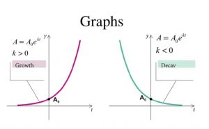
Figure 1 – Growth and Decay Figures
We always get two points for on any simple exponential graph: (0, 1) and (1, a).
In English: Exponential functions show up when the increase depends on how much is already there. For example, compound interest (the additional interest depends on how much is in the account), or simple population growth (the number of additional babies depends on how many people are in the account).
Media Attributions
- Fig1Func
