Function Applications

Steven Schlicker; David Austin; Matthew Boelkins; Margo Bergman; Dale Hoffman; David Lippman; Shana Calaway; Melonie Rasmussen

4 Function Applications

Steven Schlicker; David Austin; Matthew Boelkins; Margo Bergman; Dale Hoffman; David Lippman; Shana Calaway; and Melonie Rasmussen

Learning Objectives

By the end of this chapter students should be able to:

Explain what inverse and multivariate functions are
Explain when to transform a function and why
Give examples of different functions and their applications

Complex functions

There are several other functions that you should know something about – you should recognize their formulas and their graphs. You should know:

the absolute value functions
Higher order polynomial graphs, cubics (3rd degree) in particular
rational functions (remember vertical asymptotes?)
logarithmic functions – with base 10 and the natural log, with base e

Absolute Value Function

The absolute value of a function is the non-negative value of x without regard to its sign. It is written as follows:

$\lvert x \rvert$

Absolute Value Func

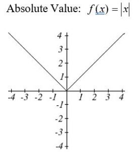
Figure 1: Absolute Value Function

Higher order polynomials

Terminology of Polynomial Functions

A polynomial is function that can be written as $f(x) = a_0+a_1x+a_2x^2+....+a_nx^n$

Each of the $a_i$ constants are called coefficients and can be positive, negative, or zero, and be whole numbers, decimals, or fractions.

A term of the polynomial is any one piece of the sum, that is any $a_ix^i$ term is a transformed power function.

The degree of the polynomial is the highest power of the variable that occurs in the polynomial.

The leading term is the term containing the highest power of the variable: the term with the highest degree.

The leading coefficient is the coefficient of the leading term.

Because of the definition of the “leading” term we often rearrange polynomials so that the powers are descending.

$f(x) = a_nx^n + .... + a_2x^2 + a_1x + a_0$

Example:

Identify the degree, leading term, and leading coefficient of the polynomial

$f(x) = 3 + 2x^2 - 4x^3$

Solution:

For the function $f(x)$ , the degree is 3, the highest power on x. The leading term is the term containing that power, $-4x^3$ . The leading coefficient is the coefficient of that term, -4.

A cubic function is a function whose highest degree term is an $x^3$ term:

Cubic Function

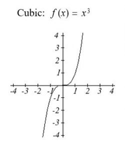
Figure 2: Cubic Function

Rational Functions

Rational functions are the ratios, or fractions, of polynomials. They can arise from both simple and complex situations.

Example:

You plan to drive 100 miles. Find a formula for the time the trip will take as a function of the speed you drive. You may recall that multiplying speed by time will give you distance. If we let t represent the drive time in hours, and v represent the velocity (speed or rate) at which we drive, then $vt= distance$ . Since our distance is fixed at 100 miles, $vt=100$ . Solving this relationship for the time gives us the function we desired:

$tv = \frac{100}{v}$

Notice that this is a transformation of the reciprocal toolkit function, $f(x) = \frac{1}{x}$ Several natural phenomena, such as gravitational force and volume of sound, behave in a manner inversely proportional to the square of another quantity. For example, the volume, $V$ , of a sound heard at a distance $d$ from the source would be related by $V = \frac{k}{d^2}$ for some constant value $k$ . These functions are transformations of the reciprocal squared toolkit function $f(x) = \frac{1}{x^2}$ .

We have seen the graphs of the basic reciprocal function and the squared reciprocal function from our review of toolkit functions. These graphs have several important features.

One over X

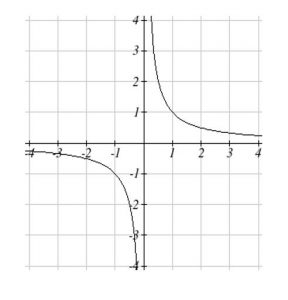
Figure 3: $f(x) = \frac{1}{x}$

One over X squared

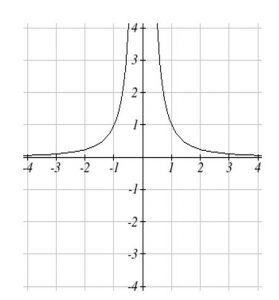
Figure 4: $f(x) =\frac{1}{x^2}$

Let’s begin by looking at the reciprocal function, $f(x) = \frac{1}{x}$ As you well know, dividing by zero is not allowed and therefore zero is not in the domain, and so the function is undefined at an input of zero.

Short Run Behavior:

As the input values approach zero from the left side (taking on very small, negative values), the function values become very large in the negative direction (in other words, they approach negative infinity).

We write: as $x \rightarrow 0^- , f(x) \rightarrow -\infty$

As we approach zero from the right side (small, positive input values), the function values become very large in the positive direction (approaching infinity).

We write: as $x \rightarrow 0^+ , f(x) \rightarrow \infty$

This behavior creates a vertical asymptote. An asymptote is a line that the graph approaches. In this case the graph is approaching the vertical line $x$ = 0 as the input becomes close to zero.

Long Run Behavior:

As the values of $x$ approach infinity, the function values approach 0.

As the values of $x$ approach negative infinity, the function values approach 0.

Symbolically: as $x \rightarrow \pm \infty , f(x) \rightarrow 0$

Based on this long run behavior and the graph we can see that the function approaches 0 but never actually reaches 0, it just “levels off” as the inputs become large. This behavior creates a horizontal asymptote. In this case the graph is approaching the horizontal line input becomes very large in the negative and positive directions.

Vertical and Horizontal Asymptotes

A vertical asymptote of a graph is a vertical line $x = a$ where the graph tends towards positive or negative infinity as the inputs approach $a$ . As $x \rightarrow a, f(x) \rightarrow \pm \infty$ .

A horizontal asymptote of a graph is a horizontal line $y=b$ where the graph approaches the line as the inputs get large. As $x \rightarrow \pm \infty, f(x) \rightarrow b$ .

Logarithmic functions

Logarithms are the inverse of exponential functions — they allow us to undo exponential functions and solve for the exponent. They are also commonly used to express quantities that vary widely in size.

Logarithm Equivalent to an Exponential

The logarithm (base b) function, written $log_b(x)$ , is the inverse of the exponential function (base b), $b^x$ .

This means the statement $b^a = c$ is equivalent to the statement $log_b (c) = a$ .

Properties of Logs: Inverse Properties

$log_b(b^x)=x$

$b^{log_bx}=x$

Example:

Write these exponential equations as logarithmic equations:

a) $2^3 = 8$

b) $5^2 = 25$

c) $10^{-4} = \frac{1}{10000}$

Solutions:

a) $log_2(8) = 3$

b) $log_5(25) = 2$

c) $log_{10}(\frac{1}{10000}) = -4$

Example:

Solve $2^x=10$ for x

Solution:

By rewriting this expression as a logarithm, we get $x = log_2 (10)$

While this does define a solution, and an exact solution at that, you may find it somewhat unsatisfying since it is difficult to compare this expression to the decimal estimate we made earlier. Also, giving an exact expression for a solution is not always useful – often we really need a decimal approximation to the solution. Luckily, this is a task calculators and computers are quite adept at. Unluckily for us, most calculators and computers will only evaluate logarithms of two bases. Happily, this ends up not being a problem, as we’ll see briefly.

Common and Natural Logarithms

The common log is the logarithm with base 10, and is typically written log(x). The natural log is the logarithm with base e, and is typically written ln(x).

Example:

Evaluate log(1000) using the definition of the common log.

Solution:

To evaluate log(1000), we can say $x=log(1000)$ , then rewrite into exponential form using the exponential form using the common log base of 10.

$10^x=1000$

From this, we might recognize that 1000 is the cube of 10, so x = 3. We also can use the inverse property of logs to write $log_{10}(10^3) = 3$

Example:

Evaluate log(500) using your calculator or computer.

Solution:

Using a computer or calculator, we can evaluate log(500) $\approx$ 2.69897

Another property provides the basis for solving exponential equations.

Properties of Logs: Exponent Property

$log_b(A^r) = r log_b (A)$

Solving exponential equations:

Isolate the exponential expressions when possible
Take the logarithm of both sides
Utilize the exponent property for logarithms to pull the variable out of the exponent
Use algebra to solve for the variable

Example:

If the function for predicting the population (in billions) of India t years after 2008 is given by using the function $f(t) = 1.14(1+0.0134)t$ . If the population continues following this trend, when will the population reach 2 billion?

We need to solve for the t so that f(t) = 2

$2 = 1.14 (1.0134)^t$

Divide by 1.14 to isolate the exponential expression

$\frac{2}{1.14} = (1.0134)^t$

Take the logarithm of both sides of the equation

$ln \frac{2}{1.14} = ln (1.0134)^t$

Apply the exponent property on the right side

$ln \frac{2}{1.14} = t ln (1.0134)$

Solve for t

$t= \frac{1.14}{ln(1.0134)} \approx \,42.23 \, years$

If this growth rate continues, the model predicts the population of India will reach 2 billion about 42 years after 2008, or approximately in the year 2050.

Graphical Features of the Logarithm

Graphically, in the function $g(x) = log_b(x)$

The graph has a horizontal intercept at (1, 0)

The graph has a vertical asymptote at x = 0

The graph is increasing and concave down

The domain of the function is x > 0, or (0, $\infty$ )

The range of the function is all real numbers, or (- $\infty$ , $\infty$ )

When sketching a general logarithm with base b, it can be helpful to remember that the graph will pass through the points (1, 0) and (b, 1).

LogGraphs

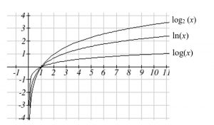
Figure 5: Graphs of logarithms

Another important observation made was the domain of the logarithm: x > 0. Like the reciprocal and square root functions, the logarithm has a restricted domain which must be considered when finding the domain of a composition involving a log.

New Functions from Old

Transformations

Changing the constants that appear in an algebraic formula changes the graph in some predictable ways.

Here are the principles:

Changing the x (the input) changes the horizontal.

Changing the y (the output) changes the vertical.

Multiplying by a constant stretches (or squashes) the graph.

Multiplying by –1 reflects the graph.

Adding a constant shifts the graph.

Here are the details:

Start with the graph of $y=f(x)$ . The graph of each of the following will have the same basic shape as $y=f(x)$ , altered as noted. For all of these, a is a constant

$y = af(x)$ is a times as tall.

$y = -f(x)$ is reflected vertically across the x-axis (upside down).

$y = f(x) + a$ is shifted up a units.

$y = f(ax)$ is $frac{1}{a}$ times as wide.

$y = f(-x)$ is reflected horizontally across the y-axis.

$y = f(x + a)$ is shifted to the left a units.

Notice that for horizontal stretches or shifts, the effect is sort of backwards from what you might expect at first. These can be confusing – check your answers by plotting a couple of points.

You can handle these all at once. You can do horizontal and vertical changes independently. For each of these, follow the order of operations – stretch and reflect first, then shift. Use the origin as your anchor point, even if it’s not on your graph.

Example: The graph of y = –4|x – 2| + 5 has the same basic shape as y = |x|. It’s been shifted to the right 2 units. It’s upside down, 4 times as tall, and has been shifted up 5 units. So the new graph has its vertex at (2, 5), opens down, and looks stretched vertically compared to the original. You can plug in a point or two to confirm your answer. The new graph goes through the point (0, –3), which makes sense. If you move 2 units to the left of the vertex, the unchanged graph goes up 2 units. Here, it goes down (because the graph is upside down) 8 units (because the graph is stretched by a factor of 4.)

Transformation

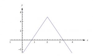
Figure 6: Transformation Function

Composition

One of the most important ways to combine functions is to chain them together, using the output from one as the input into another. A simple example of this is unit conversion – we have one function that tells us how many meters high the ball is after t seconds, and another that tells how many feet are in a certain number of meters. We can use the output of the first function (meters) as the input to the second function to find how many feet high the ball is after t seconds. The chaining together of functions in this way is called composition:

The composition of f with g, written $f \circ g(x)$ , is the function that takes x, first does g to it, and then does f to the output. That is, $f \circ g(x) = f(g(x))$

Example: Let $f(x) = 4x^2-13$ and $g(x) = \sqrt{x-2}$ .

Then their composition is $f \circ g(x)$ = $f(g(x))$ = $f(\sqrt{x-2})$ = $4({\sqrt{x-2}})^2 -13$ .

Decomposition

Sometimes you will be given the composition and be asked to identify the component pieces. This is called “decomposition.” It turns out to be a very useful skill in calculus. There are often several correct decompositions for a function, but usually only one of them is useful. It may take some practice before you can see which composition is the useful one.

Example: The function $G(x) = \frac {1}{2x+3}$ is a composition $f \circ g(x)$ . Identify the component functions f and g.

The most useful solution: In many cases, there is an “obvious” choice, which you can find by thinking about the inside and the outside. In $G(x) = \frac {1}{2x+3}$ , the “inside function” is the denominator and the “outside function” is the reciprocal function (that is, “one over”). In the composition $f \circ g(x)$ , g is the inside function and f is the outside function. So this decomposition would be $f(x) = \frac {1}{x}$ and $g(x) = 2x+3$ . Then $F(x) = f(g(x)) = f(2x+3) = \frac {1}{2x+3}$ . This is the most useful solution. This is the solution you would see in the answer pages of the textbook. This is the type of decomposition you should look for. There are usually lots of correct solutions, some of which involve some creativity to find. If you do find one, it will be correct.

Inverse Functions

The word “inverse” means backwards, and that’s what inverse functions are about – going backwards. There are a few different and useful ways to think about inverse functions.

Swapping the roles of input and output

One important reason we care about inverse functions is that, in many cases, the same relationship can give two different functions, depending on what questions you’re interested in answering. Which function you use depends on which quantity you want to use as your input.

Example: A private investigator charges a $500 fee per case, plus $80 per hour that she works on the case. There is a functional relationship between the hours she works and the amount she bills. But which is the input and which is the output?

If the number of hours she works is the input, then the number of dollars she bills is the output. And it’s a function, because each possible number of hours is associated with exactly one billing amount. This might be the function you’d think of first. If we let h be the number of hours the detective works and b be the number of dollars she bills, then this function might be written as

$b = f(h) = 500 + 80h$ .

You’d use this function if you knew how many hours she worked on your case and you wanted to know how much she would charge you.

But the very same relationship yields a different function, whose input is the billing amount and whose output is the number of hours she works. This is also a function, because each possible bill is associated with exactly one amount of time. Again, letting h be the number of hours and b be the amount she bills in dollars, we can write this function:

$h=f^{-1}(b)=\frac{b-500}{80}$

This would be a helpful function if you had a certain amount of money to spend and you wanted to know how many hours she would work on your case.

The two functions here are inverse functions. They model the same relationship, but the roles of input and output have been exchanged. That little –1 that looks like an exponent for the f in the second formula indicates it is the inverse function for f. (It is not an exponent.)

Undoing

The most important reason we want to study inverse functions is that they undo each other. Remember the algebraic definition of inverse functions:

$f(x)$ and $f^{-1}(x)$ are inverse functions means that their composition in either order is the identity function. That is, both

$f(f^{-1}(x)) = x$ and $f^{-1}(f(x)) = x$

Graphically

If you graph a function and its inverse on the same axes, the inverse will be a reflection of the original across the line y = x. That’s because the inverse function swaps the roles of input and output. On a graph, that means interchanging the order of the coordinates for every point. That is, if (x, y) is on the graph of $y = f(x)$ , then (y, x) will be on the graph of $y = f^{-1}(x)$ .

Multivariate Functions

In this and following sections, we will study functions whose input is defined in terms of more than
one variable, and then analyze these functions by looking at their graphs, calculating limits, differentiating, integrating, and more. We will see that many of the ideas from single variable calculus
translate well to functions of several variables, but we will have to make some adjustments as
well.

Example:

When people buy a large ticket item like a car or a house, they often take out a loan to make the purchase. The loan is paid back in monthly installments until the entire amount of the loan, plus interest, is paid. The monthly payment that the borrower has to make depends on the amount P of money borrowed (called the principal), the duration t of the loan in
years, and the interest rate r. For example, if we borrow $18,000 to buy a car, the monthly payment M that we need to make to pay off the loan is given by the formula: $M=\frac{1500r}{1-\frac{1}{(1+\frac{r}{12})^{12t}}}$ .The variables r and t are independent of each other, so using functional notation we write $M (r,t)=\frac{1500r}{(1-\frac{1}{1+\frac{r}{12})^{12t}}}$ .

(a) Find the monthly payments on this loan if the interest rate is 6% and the duration of the
loan is 5 years.
(b) Evaluate M(0.05, 4). Explain in words what this calculation represents.
(c) Now consider only loans where the interest rate is 5%. Calculate the monthly payments as
indicated in the table. Round payments to the nearest penny.

Duration (in years)	2	3	4	5	6
Monthly payments (in dollars)

Table 1: Monthly payments at an interest rate of 5%.

(d) Now consider only loans where the duration is 3 years. Calculate the monthly payments as indicated in the Table 1 . Round payments to the nearest penny.

Interest Rate	0.03	0.05	0.07	0.09	0.011
Monthly payments (in dollars)

Table 2: Monthly payments at an interest rate of 5%.

e) Describe as best you can the combinations of interest rates and durations of loans that
result in a monthly payment of $200.

Media Attributions

abvalue
cubicfunc
recipfunc1
recipfunc2
loggraphs
TransFunc

License

Icon for the Creative Commons Attribution-NonCommercial-ShareAlike 4.0 International License

Complex functions

Absolute Value Function

Higher order polynomials

Rational Functions

Logarithmic functions

New Functions from Old

Media Attributions

License

Share This Book