Multivariable Optimization

Margo Bergman

8 Multivariable Optimization

PreCalculus Idea — Topographical Maps

If you’ve ever hiked, you have probably seen a topographical map. Here is part of a topographic map of Stowe, Vermont, USA

(courtesy of United States Geological Survey and http://en.wikipedia.org/wiki/File:Topographic_map_example.png).

Map

Figure 1 – Topographical Map

Points with the same elevation are connected with curves, so you can read not only your east-west and your north-south location, but also your elevation. You may have also seen weather maps that use the same principle – points with the same temperature are connected with curves (isotherms), or points with the same atmospheric pressure are connected with curves (isobars). These maps let you read not only a place’s location but also its temperature or atmospheric pressure.

In this chapter, we’ll use that same idea to make graphs of functions of two variables.

Section 1: Functions of Two Variables

Real life is rarely as simple as one input – one output. Many relationships depend on lots of variables.

Example: If I put a deposit into an interest-bearing account and let it sit, the amount I have at the end of 3 years depends on P (how much my initial deposit is), r (the annual interest rate), and n (the number of compoundings per year).

Example: The air resistance on a wing in a wind tunnel depends on the shape of the wing, the speed of the wind, the wing’s orientation (pitch, yaw, and roll), plus a myriad of other things that I can’t begin to describe.

Example: The amount of your television cable bill depends on which basic rate structure you have chosen and how many pay-per-view movies you ordered.

Since the real world is so complicated, we want to extend our calculus ideas to functions of several variables.

Functions of Two Variables

If are real numbers, then is called an n-tuple. This is an extension of ordered pairs and triples. A function of n variables is a function whose domain is some set of n-tuples and whose range is some set of real numbers.

For much of what we do here, everything would work the same if we were working with 2, 3, or 47 variables. Because we’re trying to keep things a little bit simple, we’ll concentrate on functions of two variables.

A Function of Two Variables

A function of two variables is a function – that is, to each input is associated exactly one output.

The inputs are ordered pairs, (x, y). The outputs are real numbers. The domain of a function is the set of all possible inputs (ordered pairs); the range is the set of all possible outputs (real numbers).

The function can be written z = f(x,y).

Functions of two variables can be described numerically (a table), graphically, algebraically (a formula), or in English.

We will often now call the familiar y = f(x) a function of one variable.

Example: The cost of renting a car depends on how many days you keep it and how far you drive. Let d = the number of days you rent the car, and m = the number of miles you drive. Then the cost of the car rental C(d, m) is a function of two variables.

Example: The demand for hot dog buns depends on the price for the hot dog buns and also on the price for hot dogs. The demand $q_B)=f(p_B,p_D)$ is a function of two variables. (The demand for hot dogs also depends on the price of both dogs and buns).

Formulas and Tables

Just as in the case of functions of one variable, we can display a function of two variables in a table. The two inputs are shown in the margin (top row, left column), and the outputs are shown in the interior cells.

Example: Here is a table that shows the cost C(d, m) in dollars for renting a car for d days and driving it m miles:

d	m 100	200	300	400
1	55	70	85	100
2	95	110	125	140
3	135	150	165	180
4	175	190	205	220

What is the cost of renting a car for 3 days and driving it 200 miles?
What is C(100, 4)? What is C(4, 100)?
Suppose we rent the car for 3 days. Is C an increasing function of miles?

Solution:

According to the table, renting the car for 3 days (row with d = 3) and driving it 200 miles (column with m = 300) will cost $150 (highlighted in aqua).
Careful now – the input is an ordered pair, so in C(100, 4), the 100 has to be a value of d and the 4 has to be a value of m. C(100, 4) would be the cost of renting a car for 100 days and driving it 4 miles. That cost is not in the table. (And that would be a pretty silly way to rent a car.) On the other hand, C(4, 100) is the cost of renting for 4 days and driving 100 miles – the table says that would cost $175.
If we know that d is fixed at 3, we’re looking at C(3, m). This is now a function of 1 variable, just m. We can see the table that displays values of this function by focusing our attention on just the row where d = 3:

d	m 100	200	300	400
3	135	150	165	180

Now we can see that if we rent for 3 days, the cost appears to be an increasing function of the number of miles we drive. (That shouldn’t have been surprising.)

The idea of fixing one variable and watching what happens to the function as the other varies will come up again and again.

It’s hard to display a function of more than two variables in a table. But it’s convenient to work with formulas for functions of two variables, or as many variables as you like.

Example: The cost C(d,m) in dollars for renting a car for d days and driving it m miles is given by the formula $C(d,m) = 40d+.15m$

What is the cost of renting a car for 3 days and driving it 200 miles?
What is C(100, 4)? What is C(4, 100)?
Suppose we rent the car for 3 days. Is C an increasing function of miles?

Solution:

$C(3,200) = 40(3)+.15(200)=$150$ . This is the same value we got from the table. The formula will give us the same answers for any of the table values.
C(100, 4) makes perfect sense to the formula (even if it doesn’t make sense for actually renting a car). So now we can get an answer. To rent the car for 100 days and drive it for 4 miles should cost $4000.60. C(4, 100) = $175, as before.
If we fix d = 3, then C(d, m) becomes C(3, m) = 40(3) + .15m = 120 + .15m. Yes, this is an increasing function of m; I can tell because it’s linear and its slope is .15 > 0.

Reality check – the formula that gives the cost for the rental car makes sense for all values of d and m. But that’s not how the real cost works – you can’t rent the car for a negative number of days or drive a negative number of miles. (That is, there are domain restrictions.) In addition, most car rental agreements don’t compute a charge for fractions of days; they round up to the next whole number of days.

Example: Let $f(x,y,z,w)=35x^2w-\frac{1}{z}+yz^2$ . Evaluate $f(0,1,2,3)$ .

Solution: Remember that this is an ordered 4-tuple; make sure the numbers get substituted into the correct places:

$f(0,1,2,3)=35*0^2*3-\frac{1}{2}+1*2^2=3.5$ .

Graphs – Contour Diagrams

The graph of a function of two variables is a surface in three-dimensional space. Think of each input (x,y) as a location on the plane, and plot the point f(x,y) units above that point. But how do you draw a picture of the surface?

You can use a fancy computer program to draw beautiful perspective drawings.

CountourDiag

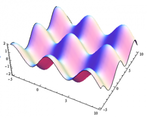
Figure 2 – Contour Diagram

You can try to draw a perspective drawing by hand. I’m very bad at this.
But one of the best ways, the way I like best, the way we will concentrate on here, is using level curves to draw contour diagrams. A contour diagram is like a topographical map – points with the same elevation (outputs) are connected with curves. Each particular output is called a level, and these curves are called level curves or contours. The closer the curves are to each other, the steeper that section of the surface is. Topographical maps give hikers information about elevation, steep and shallow grades, peaks and valleys. Contour diagrams give us the same kind of information about a function.

ContourDiag2

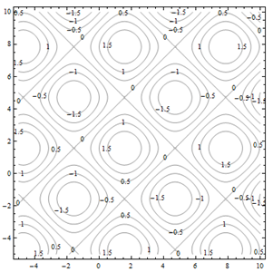
Figure 3 – Contour Diagram 2

This is a contour diagram of the same surface shown in Fig. 2. The level curves are graphs in the xy-plane of curves f(x, y) = c for various constants c.

Each of the squares corresponds to one of the bumps on the surface. If the contours are positive, as highlighted in Fig. 4, the bump is above the xy-plane. If the contours are negative, the bump extends below the xy-plane.

ContourDiag3

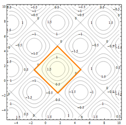
Figure 4 – Contour Diagram 3

Everywhere on the crisscrossed pattern of diagonal lines, the height of the surface is 0, so the surface is on the xy-plane. This is a feature that I couldn’t see when I looked at the perspective drawing.

ContourDiag4

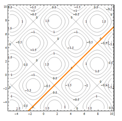
Figure 5 – Contour Diagram 4

Example: Here is the contour diagram for our car rental example. I made it by setting the cost function $C(d,m)=40d+.15m=c$ for c = 0, 100, 200, 300, and 400 and drawing the curves in the dm-plane.

Diagram5

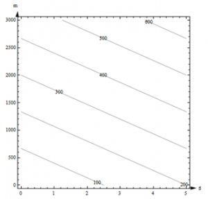
Figure 6 – Car Rental Contour Diagram

The first coordinate of the ordered pair is d, so the d-axis will be horizontal; the m-axis will be vertical. Remember that the domain for this function is really just where d ≥ 0 and m ≥ 0, so I only drew the curves in the first quadrant.

For c = 0:

$C(d,m)=40d+.15m=c$

$-40d=.15m$

$m=-\frac{40}{.15}d\cong-267d$

This is the equation of a line, with slope about, passing through the origin. Because of the domain restrictions, the “curve” I will draw for this level is simply the origin.

Putting this back into the car rental context, the only point where I pay $0 for renting the car is when I rent the car for 0 days and drive it 0 miles – that is, if I don’t rent it at all.

For c = 100:

$C(d,m)=40d+.15m=100$

$-40d+100=.15m$

$m=-\frac{40}{.15}d+\frac{100}{.15}\cong-267d+667$

This is the equation of a line, with slope about, and d-intercept of about 667. This section of this line that lies in the first quadrant is shown with 100 labeling it.

Putting this into context, any point on that line represents a (d, m) combination of days and miles that will make the cost exactly $100. So, for example – if I rent the car for 0 days and drive it 667 miles, it will cost me $100. If I rent the car for 2.5 days and don’t drive any miles, it will cost me $100.

For c = 200, c = 300, and so on? I can see the pattern now. Each of these level curves will have the same slope, but the m-intercept will increase each time. The contour diagram is a bunch of equally spaced parallel lines.

Example: The contour diagram for the cost C(d,m) in dollars for renting a car for d days and driving it m miles is shown in Fig. 6. Use the diagram to answer the following questions.

What is the cost of renting a car for 3 days and driving it 200 miles?
What is C(100, 4)? What is C(4, 100)?
Suppose we rent the car for 3 days. Is C an increasing function of miles?

Solution:

The point (3, 200) is between contours on this graph, so I can’t get an exact answer for C(3, 200). (But it’s typical for a graph that we would have to estimate). It looks to me as if (3, 200) is halfway between the 100 and the 200 contours, so I will estimate that C(3, 200) is about $150.
Estimates from the graph are necessarily very rough. The graph only shows a little information (in this way, a contour diagram is like a table), so I have to extrapolate in between. But for most graphs, I don’t actually know what happens between the contours. All I know for sure is that the output at (3, 200) is between the two levels I see. For this car rental example, I also know a formula, and my table showed this particular input, so I have other ways to get a better answer.
I can’t find (100, 4) on this diagram, so I can’t make an estimate of C(100, 4) from this graph.(4, 100) lies between the contours for 100 and 200. It looks closer to 200, so I’ll estimate that C(4, 100) is about $180.
If we fix d = 3, we get a vertical line. What happens as m increases on this vertical line? As m increases, the function values shown on the contours increase – C appears to be an increasing function of miles.

ContourDiag6

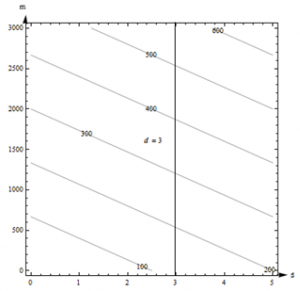
Figure 7 – Car Rental Example Contour

Example: Here is a contour diagram for a function g(x,y).

ContourDiag7

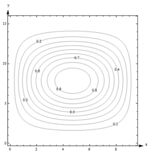
Figure 8 – Function g(x,y)

Use the diagram to answer the following questions:

What is g(3, 5)?
What is the highest point shown on the diagram? What is the lowest point shown?
If you start at (3, 5) and head in the positive x direction, do you go uphill or downhill first?

Solution: 1. g(3, 5) is 0.6. I can tell because the point is right on one of the contours.

ContourDiag8

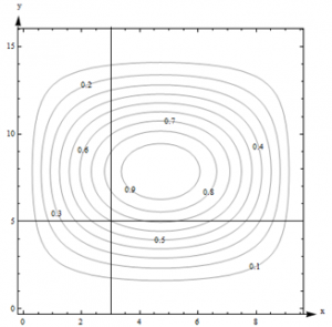
Figure 9 – Function g(x,y) – Solution

2. The highest contour shown is 0.9, and there would be a contour for 1.0 if the surface had ever got that high. However, the height seems to be increasing as we move in toward the center, so I’m guessing that the g gets to nearly 1 in the center. The lowest contour is 0.1. But again, I will guess that the height continues to decrease, so I think g is nearly 0 around the outside.

3. Starting at the point (3, 5, 0.6) on the surface and traveling to the right along the horizontal line shown in Fig. 9, you would cross the contour for 0.7 next. So the function increases first (we go uphill), and then decreases again.

Note one more time – we don’t really know what happens between the contours. All we can do is estimate from the information in the graph.

Example: Here is a contour diagram for a function F(x,y).

ContourDiag9

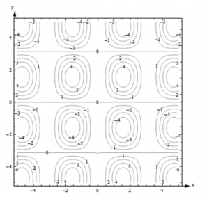
Figure 10 – Function F(x,y)

Describe the surface shown in Fig. 10.
Suppose you travel along the surface in the positive y-direction, starting on the surface at the point above (or below) the point (x, y) = (-1, 1). Describe your journey.

Solution:

The surface is bumpy, with regularly spaced oval bumps. Notice that some of the bumps go up (positive contours), but others go down. Between the bumps, there are horizontal lines that are completely level, with an elevation of 0.
It looks as if F(-1,1) is about 3. As I head in the positive y-direction along the line shown in Fig. 11, I first go uphill, nearly to 4, then I start going downhill. As I keep going north, I keep descending, going into the dip, until nearly -4. I’m starting to go uphill again just as I leave the graph.

ContourDiag10

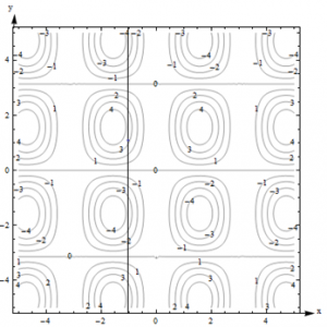
Figure 11 – Function F(x,y) – Solution

What happens if you have a function of more than two variables? Its graph will be a hyper-surface. For example, the graph of a function of four variables will be a hyper-surface in 5-dimensional space. This is hard (impossible for most of us) to visualize. Even the contours are hard to visualize – instead of curves in the plane, they’re hyper-surfaces in 4-dimensional space. So – if you have more than two variables, the graph isn’t usually very useful.

Functions of Two Real-Life Variables

Complementary goods and substitute goods

The demand for some pairs of goods have a relationship, where the quantity demanded for one product depends somehow on the prices for both.

Two goods are complementary if an increase in the price of either decreases the demand for both.

Example: The demand for cars depends on both the price for cars and the price of gasoline.

Example: The demand for hot dog buns depends on both the price for the buns and the price for the hot dogs.

Two goods are substitutes if an increase in the price of one increases the demand for the other.

Example: The demand for Brand A depends on its price and also on the price of its main competitor Brand B. If the Brand B raises its price, consumers will switch brands – substitute – and demand for Brand A will increase.

Think brands of soft drinks, detergent, or paper towels. A traditional example is coffee and tea – the idea is that consumers are simply looking for a hot drink and they’ll buy whatever is cheaper. But this has always seemed fishy to me – I’ve never met any coffee- or tea-drinkers who would happily switch.

These demand functions are functions of two variables.

Example: The demand functions for two products are given below. p1, p2, q1, and q2 are the prices (in dollars) and quantities for products 1 and 2.

$q_1=200-3p_1-p_2$

$q_2=150-p_1-2p_2$

Are these two products complementary goods or substitute goods? What is the quantity demanded for each when the price for product 1 is $20 per item and the price for product 2 is $30 per item?

Solution: These products are complementary – an increase in either price decreases both demands. You can see that because the coefficients are both negative in each demand function.

When $p_1 = 20$ and $p_2 = 30$ , we have

$q_1=200-3*(20)-(30)=110$

$q_2=150-20-2*(30)=70$

110 units are demanded for product 1 and 70 units are demanded for product 2 when the price for product 1 is $20 per item and the price for product 2 is $30 per item.

Cobb-Douglas Production function

Production functions are used to model the total output of a firm for a variety of inputs (doesn’t this sound like a function of several variables?). One example is a Cobb-Douglas Production function:

$P=AL^\alpha K^\beta$

In this function, P is the total production, A is a constant, $\alpha$ and $\beta$ are constants between 0 and 1, L is the labor force, and K is the capital expenditure. (And the units must be massaged well.)

You can read more about Cobb-Douglas Production functions at http://en.wikipedia.org/wiki/Cobb-Douglas. You can read about other kinds of production functions at http://en.wikipedia.org/wiki/Production_function.

Section 2: Calculus of Functions of Two Variables

Now that you have some familiarity with functions of two variables, it’s time to start applying calculus to help us solve problems with them. In Chapter 2, we learned about the derivative for functions of two variables. Derivatives told us about the shape of the function, and let us find local max and min – we want to be able to do the same thing with a function of two variables.

First let’s think. Imagine a surface, the graph of a function of two variables. Imagine that the surface is smooth and has some hills and some valleys. Concentrate on one point on your surface. What do we want the derivative to tell us? It ought to tell us how quickly the height of the surface changes as we move …. Wait, which direction do we want to move? This is the reason that derivatives are more complicated for functions of several variables – there are so many directions we could move from any point.

It turns out that our idea of fixing one variable and watching what happens to the function as the other changes is the key to extending the idea of derivatives to more than one variable.

Partial Derivatives

Suppose that z = f(x, y) is a function of two variables.

The partial derivative of f with respect to x is the ordinary derivative of the function f(x,y) where we think of x as the only variable and act as if y is a constant.

The partial derivative of f with respect to y is the ordinary derivative of the function f(x,y) where we think of y as the only variable and act as if x is a constant.

The “with respect to x” or “with respect to y” part is really important – you have to know and tell which variable you are thinking of as THE variable.

Geometrically – the partial derivative with respect to x gives the slope of the curve as you travel along a cross-section, a curve on the surface parallel to the x-axis. The partial derivative with respect to y gives the slope of the cross-section parallel to the y-axis.

Notation for the Partial Derivative:

The partial derivative of y = f(x) with respect to x is written as

$f_x(x,y)$ or $z_x$ simply $f_x$

The Leibniz notation is $\frac{\delta f }{dx}$ , or $\frac{\delta z}{dx}$

We use an adaptation of the $\frac{\delta z}{dx}$ notation to mean “find the partial derivative of f(x,y) with respect to x:”

$\frac{\delta}{\delta x}(f(x,y))$ , or $\frac{\delta f}{\delta x}$

To estimate a partial derivative from a table or contour diagram:

The partial derivative with respect to x can be approximated by looking at an average rate of change, or the slope of a secant line, over a very tiny interval in the x-direction (holding y constant). The tinier the interval, the closer this is to the true partial derivative.

To compute a partial derivative from a formula:

If f(x,y) is given as a formula, you can find the partial derivative with respect to x algebraically by taking the ordinary derivative thinking of x as the only variable (holding y fixed).

Of course, everything here works the same way if we’re trying to find the partial derivative with respect to y – just think of y as your only variable and act as if x is constant.

The idea of a partial derivative works perfectly well for a function of several variables – you focus on one variable to be THE variable and act as if all the other variables are constants.

Example: Here is a contour diagram for a function g(x,y). Use the diagram to answer the following questions:

Estimate $g_x(3,5)$ and $g_y(3,5)$
Where on this diagram is $g_x$ greatest? Where is $g_y$ greatest?

Contour11

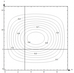
Figure 12 – Function g(x,y)

Solution:

$g_x(3,5)$ means I’m thinking of x as my only variable, so I’ll hold y fixed at y = 5. That means I’ll be looking along the horizontal line y = 5. (3, 5) lies on the contour line, so I know that g(3, 5) = 0.6. I’ll use the next point that I can read as I move to the right – that would be g(4.2,5) = 0.7. Then I’ll find the average rate of change:

Average rate of change = (change in output) / (change in input) = $\frac{\Delta g}{\Delta x} = \frac{0.7-0.6}{4.2-3} = \frac{1}{12}\cong .083$ .

I can do the same thing by going to the next point I can read to the left, which is g(2.4,5) = 0.5. Then the average rate of change is $\frac{\Delta g}{\Delta x} = \frac{0.5-0.6}{2.4-3} = \frac{1}{6}\cong .167$ . Either of these would be a fine estimate of $g_x(3,5)$ given the information we have, or you could take their average. I estimate that $g_x(3,5) \cong.125$ .

Estimate $g_y(3,5)$ the same way, but moving on the vertical line. Using the next point up, I get the average rate of change = $\frac{\Delta g}{\Delta y} = \frac{0.7-0.6}{5.8-5} = .125$ . Using the next point down, I get $\frac{\Delta g}{\Delta y} = \frac{0.5-0.6}{4.5-5} = .2$ . Taking their average, I estimate $g_y(3,5)\cong .1625$ .

2. $g_x$ means x is my only variable, and I’m thinking of y as a constant. So I’m thinking about moving across the diagram on horizontal lines. $g_x$ will be greatest when the contour lines are closest together, when the surface is steepest – then the denominator in $\frac{\Delta g}{\Delta x}$ will be small, so will $\frac{\Delta g}{\Delta x}$ be big. Scanning the graph, I can see that the contour lines are closest together when I head to the left or to the right from about (0.5, 8) and (9, 8). So $g_x$ is greatest at about (0.5, 8) and (9, 8). For $g_y$ , I want to look at vertical lines. $g_y$ is greatest at about (5, 3.8) and (5, 12).

Example: Cold temperatures feel colder when the wind is blowing. Windchill is the perceived temperature, and it depends on both the actual temperature and the wind speed – a function of two variables! You can read more about windchill at http://www.nws.noaa.gov/om/windchill/. Fig. 13 shows a table (courtesy of the National Weather Service) that shows the perceived temperature for various temperatures and windspeeds. Note that they also include the formula, but I want to use the information in the table.

Contour12

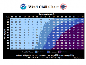
Figure 13 – Wind Chill Chart

What is the perceived temperature when the actual temperature is 25˚F and the wind is blowing at 15 miles per hour?
Suppose the actual temperature is 25˚F. Use information from the table to describe how the perceived temperature would change if the wind speed increased from 15 miles per hour?

Solution:

Reading the table, we see that the perceived temperature is 13˚F.
This is a question about a partial derivative. We’re holding the temperature (T) fixed at 25˚F, and asking what happens as wind speed (V) increases from 15 miles per hour. We’re thinking of V as the only variable, so we want $WindChill_V$ = $W_V$ when T = 25 and V = 15. We’ll find the average rate of change by looking in the column where T = 25 and letting V increase, and use that to approximate the partial derivative.

$W_V\cong\frac{\Delta W}{\Delta V}=\frac{11-13}{20-15}=-0.4$

What are the units? W is measured in ˚F and V is measured in mph, so the units here are ˚F/mph. And that lets us describe what happens:

The perceived temperature would decrease by about .4˚F for each mph increase in wind speed.

Example: Find $f_x$ and $f_y$ at the points (0, 0) and (1, 1) if $f(x,y) = x^2-4xy+4y^2$

Solution: To find $f_x$ , take the ordinary derivative of f with respect to x, acting as if y is constant:

$f_x(x,y) = 2x-4y$

Note that the derivative of the $4y^2$ term with respect to x is zero – it’s a constant.

Similarly, $f_y(x,y) = -4x+8y$ . Now we can evaluate these at the points:

$f_x(0,0) = 0$ and $f_y(0,0) = 0$ ; this tells us that the cross sections parallel to the x- and y- axes are both flat at (0,0).

$f_x(1,1) = -2$ and $f_y(1,1) = 4$ ; this tells us that above the point (1, 1), the surface decreases if you move to more positive x values and increases if you move to more positive y values.

Example: Find $\frac{\delta f}{\delta x}$ = $\frac{\delta f}{\delta y}$ if $f(x,y)=\frac{e^x+y}{y^3+y}+y(ln y)$

Solution: $\frac{\delta f}{\delta x}$ means x is our only variable, we’re thinking of y as a constant. Then we’ll just find the ordinary derivative. From x’s point of view, this is an exponential function, divided by a constant, with a constant added. The constant pulls out in front, the derivative of the exponential function is the same thing, and we need to use the chain rule, so we multiply by the derivative of that exponent (which is just 1):

$\frac{\delta f}{\delta x}=\frac{1}{y^3+y}e^x+y$

$\frac{\delta f}{\delta x}$ means that we’re thinking of y as the variable, acting as if x is constant. From y’s point of view, f is a quotient plus a product – we’ll need the quotient rule and the product rule:

$\frac{\delta f}{\delta y}=\frac{()()-()()}{{}^2}+()()+()()$

=

$=\frac{(e^x+y(1))(y^3+y)-(e^x+y)(3y^2+1)}{(y^3+y)^2}+(1)(ln y)+(y)(\frac{1}{y})$

For goodness’ sake, don’t try to simplify that. Just leave it.

Example: Find if $f_x if f(x,y,z,w) = 35x^2x-\frac{1}{z}+yz^2$

Solution: $f_z$ means z is our only variable, so we’ll act as if all the other variables (x, y and w) are constants and take the ordinary derivative.

$f_z if f(x,y,z,w) = \frac{1}{z^2}+2yz$

Section 2: Optimization

The partial derivatives tell us something about where a surface has local maxima and minima. Remember that even in the one-variable cases, there were critical points which were neither maxima nor minima – this is also true for functions of many variables. In fact, as you might expect, the situation is even more complicated.

Second Derivatives

When you find a partial derivative of a function of two variables, you get another function of two variables – you can take its partial derivatives, too. We’ve done this before, in the one-variable setting. In the one-variable setting, the second derivative gave information about how the graph was curved. In the two-variable setting, the second partial derivatives give some information about how the surface is curved, as you travel on cross-sections – but that’s not very complete information about the entire surface.

Imagine that you have a surface that’s ruffled around a point, like what happens near a button on an overstuffed sofa, or a pinched piece of fabric, or the wrinkly skin near your thumb when you make a fist. Right at that point, every direction you move, something different will happen – it might increase, decrease, curve up, curve down. A simple phrase like “concave up” or “concave down” can’t describe all the things that can happen on a surface.

Surprisingly enough, though, there is still a second derivative test that can help you decide if a point is a local max or min or neither. So we still do want to find second derivatives.

Second Partial Derivatives

Suppose $f(x,y)$ is a function of two variables. Then it has four second partial derivatives:

$f_xx = \frac{\delta}{\delta x}(f_x) = (f_x)_x$ and

$f_xy = \frac{\delta}{\delta y}(f_x) = (f_x)_y$ and

$f_yx = \frac{\delta}{\delta y}(f_x) = (f_x)_y$ and

$f_yy = \frac{\delta}{\delta y}(f_y) = (f_y)_y$ and

and are called the mixed (second) partial derivatives of f

Example: Find all four partial derivatives of $f(x,y) = x^2-4xy+4xy^2$

Solution: We have to start by finding the (first) partial derivatives:

$f_x(x,y) = 2x-4y+4y^(2)$

$f_y(x,y) = -4x+8yx$

Now we’re ready to take the second partial derivatives:

$f_xx (x,y)= \frac{\delta}{\delta x}(2x-4y) = 2$

$f_xy (x,y)= \frac{\delta}{\delta y}(2x-4y) = -4$

$f_yx (x,y)= \frac{\delta}{\delta x}(-4x+8y) = -4$

$f_yy (x,y)= \frac{\delta}{\delta y}(-4x+8y) = 8$

You might have noticed that the two mixed partial derivatives were equal in this last example. It turns out that it’s not a coincidence – it’s a theorem.

Mixed Partial Derivative Theorem

If $f$ , $f_x$ , $f_y$ , $f_xy$ , and $f_yx$ are all continuous (no breaks in their graph)

Then= $f_xy$ = $f_yx$ .

In fact, as long as f and all its appropriate partial derivatives are continuous, the mixed partials are equal even if they are of higher order, and even if the function has more than two variables.

This theorem means that the confusing Leibniz notation for second derivatives is not a big problem – in almost every situation, the mixed partials are equal, so it doesn’t matter in which order we compute them.

Example: Find $\frac{\delta^2 f}{\delta x \delta y}$ for $f(x,y) = \frac{e^x+y}{y^3+y}+y(ln y)$

Solution: We already found the first partial derivatives in an earlier example:

$\frac{\delta f}{\delta y}=\frac{()()-()()}{{}^2}+()()+()()$

=

$=\frac{(e^x+y(1))(y^3+y)-(e^x+y)(3y^2+1)}{(y^3+y)^2}+(1)(ln y)+(y)(\frac{1}{y})$

Now we need to find the mixed partial derivative – the Theorem says it doesn’t matter whether we find the partial derivative of $\frac{\delta f}{\delta x} = \frac{1}{y^3+y}e^x+y$ with respect to y or the partial derivative of $\frac{\delta f}{\delta y} = \frac{(e^x+y(1))(y^3+y)-(e^x+y)(3y^2+1)}{(y_3+y)_2} +(1)(ln y) + (y)(\frac{1}{y})$ with respect to x. Which would you rather do?

Yes, me too. I’ll compute the mixed partial by finding the partial derivative of $\frac{\delta f}{\delta x} = \frac{1}{y^3+y}e^x+y$ with respect to y – it still looks messy, but it looks less messy:

$\frac{\delta_2 f}{\delta x \delta y} = \frac{\delta_2 f}{\delta y \delta x} = \frac{\delta}{\delta y} \left(\frac{1}{y^3+y}e^x+y \right) = \frac{(e^e+y)(y^3+y)-(e^x+y)(3y^2+1)}{(y^3+y)_2}$

If you’d decided to do this the other way, you’d end up in the same place. Eventually.

Local Maxima, Minima, and Saddle Points

Let’s briefly review max-min problems in one variable.

A local max is a point on a curve that is higher than all the nearby points. A local min is lower than all the nearby points. We know that local max or min can only occur at critical points, where the derivative is zero or undefined. But we also know that not all critical points are max or min, so we also need to test them, with the First Derivative or Second Derivative Test.

The situation with a function of two variables is much the same. Just as in the one-variable case, the first step is to find critical points, places where both the partial derivatives are either zero or undefined.

Definition:

f has a local maximum at (a, b) if f(a, b) ≥ f(x, y) for all points (x, y) near (a, b)

f has a local minimum at (a, b) if f(a, b) ≤ f(x, y) for all points (x, y) near (a, b)

A critical point for a function f(x, y) is a point (x, y) (or (x, y, f(x, y)) where both the following are true:

$f_x$ =0 or is undefined

and

$f_y$ =0 or is undefined

Useful Fact: Just as in the one-variable case, a local max or min of f can only occur at a critical point.

And then, just as in the one-variable setting, not all critical points are local max or min. For a function of two variables, the critical point could be a local max, local min, or a saddle point.

A point on a surface is a local maximum if it’s higher than all the points nearby; a point is a local minimum if it’s lower than all the points nearby.

A saddle point is a point on a surface that is a minimum along some paths and a maximum along some others. It’s called this because it’s shaped a bit like a saddle you might use to ride a horse. You can see a saddle point by making a fist – between the knuckles of your index and middle fingers, you can see a place that is a minimum as you go across your knuckles, but a maximum as you go along your hand toward your fingers.

Here is a picture of a saddle point from a few different angles. This is the surface $f(x,y) = 5x^2-3y^2+10$ , and there is a saddle point above the origin. The lines show what the surface looks like above the x– and y-axes. Notice how the point above the origin, where the lines cross, is a local minimum in one direction, but a local maximum in the other direction.

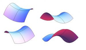
Figure 15 – Saddle Points

Second Derivative Test

Just as in the one-variable case, we’ll need a way to test critical points to see whether they are local max or min. There is a second derivative test for functions of two variables that can help – but, just as in the one-variable case, it won’t always give an answer.

The Second Derivative Test for Functions of Two Variables:

Find all critical points of f(x,y).

Compute $D = (f_xx)(f_yy) - (f_xy)(f_yx)$ , and evaluate it at each critical point.

(a) If D > 0, then f has a local max or min at the critical point. To see which, look at the sign of $f_xx$ :

If $f_xx$ > 0, then f has a local minimum at the critical point.

If $f_xx$ < 0, then f has a local maximum at the critical point.

(b) If D < 0 then f has a saddle point at the critical point.

(c) If D = 0, there could be a local max, local min, or neither.

Example: Find all local maxima, minima, and saddle points for the function $f(x,y) = x^3 + y^3 + 3x^2 - 3y^2 - 8$

Solution: First we need the critical points:

$f_x = 3x^2 + 6x$

and

$f_y = 3y^2 - 6y$

Critical points are the places where both these are zero (neither is ever undefined):

$f_x = 3x^2 + 6x$ = $3x(x+2)$ = 0 when x = 0 or when x = −2.

$f_y = 3y^2 - 6y$ = $3y(y-2)$ = 0 when y = 0 or when y = 2.

Putting these together, we get four critical points: (0, 0), (−2, 0), (0, 2), and (−2, 2).

Now to classify them, we’ll use the Second Derivative Test. We’ll need all the second partial derivatives:

$f_xx = 6x+6$

$f_yy = 6y-6$

$f_xy = 0 = f_yx$

Then $D = (6x+6)(6y-6)-(0)(0) = (6x+6)(6y-6)$ .

Now look at each critical point in turn:

At (0, 0): $D = (6*0+6)(6*0-6) = (6)(-6)=-36 < 0$ ; there is a saddle point at (0, 0).

At (−2, 0): $D = (6*(-2)+6)(6*(0)-6) = (-6)(-6)=36 > 0$ , and ; there is a local maximum at (−2, 0).

At (0, 2): $D = (6)(6)=36 > 0$ and $f_xx = 6 >0$ ; there is a local minimum at (0, 2).

At (−2, 2): $D = (-6)(6)= < 0$ ; there is another saddle point at (−2, 2).

Example: Find all local maxima, minima, and saddle points for the function:

$z=9x^3+\frac{y^3}{3}-4xy$

Solution: We’ll need all the partial derivatives and second partial derivatives, so let’s compute them all first:

$z_x = 27x^2-4y$ ;

$z_y = y^2-4x$ ;

$z_xx = 54x$ ;

$z_yy = 2y$ ;

$z_xy = -4 = z_yx$ ;

Now to find the critical points: We need both $z_x$ and $z_y$ to be zero (neither is ever undefined), so we need to solve this set of equations simultaneously:

$z_x = 27x^2-4y = 0$

$z_y = y^2-4x$

Perhaps it’s been a while since you solved systems of equations. Just remember the substitution method – solve one equation for one variable and substitute into the other equation:

$27x^2-4y$ and $y^2-4x$ -> solve $y^2-4x = 0$ for $x=\frac{y^2}{4}$ , then substitute into the other equation:

$27 \left( \frac{y^2}{4} \right)^2 - 4y = 0$

$\frac{27}{16}y^4-4y = 0$

Now we have just one equation in one variable to solve. You can use algebra (this one factors, it’s not too bad), or you can use technology to find the solutions: $y = 0$ or $y=\frac{4}{3}$ . Plugging back in to find x gives us the two critical points: (0, 0) and $(\frac{4}{9},\frac{4}{3})$ .

Now to test them: Compute $D = (f_xx)(f_yy) - (f_xy)(f_yx)$ , evaluate it at the two critical points, and see:

At (0,0): D = −16 < 0, so there is a saddle point at (0, 0).

At $(\frac{4}{9},\frac{4}{3}): D = 48 > 0$ , and $f_xx$ > 0 , so there is a local minimum at $(\frac{4}{9},\frac{4}{3})$ .

Applied Optimization

Example: A company makes two products. The demand equations for the two products are given below. p1, p2, q1,and q2 are the prices and quantities for products 1 and 2.

$q_1=200-3p_1-p_2$

$q_2=150-p_1-2p_2$

Find the price the company should charge for each product in order to maximize total revenue. What is that maximum revenue?

Solution: Revenue is still price × quantity. If we’re selling two products, the total revenue will be the sum of the revenues from the two products:

$p_1q_1 + p_2q_2 = p_1(200-3p_1-p_2)+p_2(150-p_1-2p_2)$

$R(p_1,p_2)=200p_1-3p^2_1-2p_1p_2+150p_2-2p^2_2$

This is a function of two variables, the two prices, and we need to optimize it – just as in the previous examples.

Find critical points (now the notation here gets a bit hard to look at, but hang in there – this is the same stuff we’ve done before): $R_p_1 = 200-6p_1-2p_2$ and $R_p_2 = 150-2p_1-4p_2$