Simple Carbon Cycle Models
Industrial activity has resulted in the release of over 2.2 trillion metric tons of carbon dioxide into the atmosphere. The first trillion tons took centuries. The most recent trillion was emitted in only 30 years. What happens to all that carbon dioxide after it’s emitted? Unlike gases like methane, which dissipate on decadal timescales, much of the carbon dioxide that’s emitted now will be in the air centuries from now. Some will even be in the atmosphere hundreds of thousands of years from now.
Not all fossil carbon dioxide that’s emitted stays in the air; some is taken up in land ecosystems, as higher CO2 levels cause an increase in photosynthesis. However, flux of carbon dioxide out of the land from soil respiration also increases in a warmer world, as microbial activity speeds up. In the ocean, more CO2 can dissolve into seawater when there’s more of the gas in the air above. However this causes ocean acidification, due to increased concentration of carbonic acid.
Emissions-Forced Tests
Despite the importance of the carbon cycle, most of the scenarios run in CMIP are not actually forced by emissions. CMIP6’s ScenarioMIP, for instance, are concentration-forced runs, with the exception of the very high emissions esm-ssp585 experiment. The standard scenarios are instead forced with heat-trapping gas concentrations created from the MAGICC reduced-complexity model.
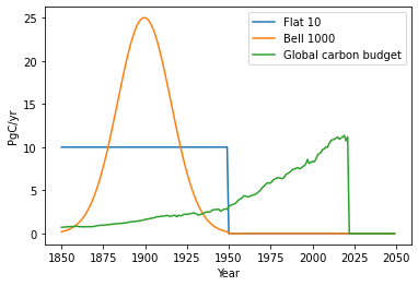
There are a few emissions-forced tests that have been created for CMIP, and are under consideration for CMIP7. First is the pulse100 experiment, a pulse emission of 100 GtC in year 0, followed by zero emissions. We’ll consider other pulse amplitude experiments in this study as well, including pulse1000 and pulse500. Second is the flat10 experiment, which consists of 10 GtC/yr emissions applied for 100 years, followed by zero emissions. Third is the esm-bell-1000PgC experiment, which is 1000 PgC applied in a bell-curve over a 100 year period, with zero emissions afterwards. The sigma parameter for the bell curve is chosen to be 100/6, so that the emissions span 3 standard deviations about the center. These emissions of the latter two cases are plotted below, along with the historical emissions since 1850 from the Global Carbon Budget (which total 675 PgC through 2022). In these idealized experiments, all other emissions are set to zero. Note that the pulse1000, flat10, and esm-bell-1000PgC experiments all have cumulative carbon emissions of 1000 PgC.
Let’s examine some of the ways the carbon cycle is parameterized within simple models, and study their response to these simple emissions-forced tests. We’re doing this in order to better understand what might happen in the future, including all relevant uncertainties, and to learn more about the physical processes that determine where all the carbon goes.
Impulse-Response Model (Joos et al 2013)
This simple carbon cycle model was developed in a large collaborative study with 28 authors from 10 different countries across the world (Joos et al 2013). They compared the results from carbon cycle models of a range of complexity, and used these results to create simple parameterizations.
There were 15 models that participated in the intercomparison: only 3 state-of-the-art Earth system models (ESMs), along with 7 Earth system models of intermediate complexity (EMICs) and 4 box models. The models are run with a pulse of 100 GtC (366 GtCO2, equivalent to around 10 years of current emissions) added to a background climate with 389 ppm CO2 (the concentration in 2010). The carbon cycle state in 2010 is calculated by running a first simulation with CO2 concentrations prescribed to the observed historical values, and calculating the emissions needed in the model to generate the observed CO2 levels. Then a new simulation is run with those calculated emissions, and the pulse is added in 2010 to that simulation.
Following the pulse, the ESMs were run for 101 or 289 years (not very long!), while the other models were run for 585-1000 years. Then the fraction of carbon that remains as a function of time is calculated, as well as accompanying information like the global temperature change, ocean heat content, sea level rise, and carbon uptake in the land and ocean.
The following equation was derived from the multi-model mean atmospheric carbon dioxide response to the emissions pulse P:
[latex]C(t)/P = a_0 + \sum_\limits{i=1}^{3}\ a_i\ e^{-t/\tau_i}[/latex]
where
| Box | 0 | 1 | 2 | 3 |
| Fraction a | 0.22 | 0.22 | 0.28 | 0.28 |
| Timescale τ | infinity | 390 yrs | 37 yrs | 4.3 yrs |
| Interpretation | chemical weathering on land | deep ocean carbon uptake | land carbon uptake | surface ocean carbon uptake |
and C0 is the initial pulse amplitude (potentially using the expression 1 ppm CO2 = 2.1 GtC to change units). Atmospheric carbon dioxide concentration anomaly is calculated by adding the 4 boxes, i.e., [latex]C(t) = \sum_\limits{i=0}^3\ C_i(t)[/latex]. The a coefficients add up to 1, because this is a partitioning of the initial pulse into 4 boxes. Subsequent decreases in the CO2 in each box represent uptake from the atmosphere into land or ocean.
So in this model, 22% percent of the carbon dioxide in the pulse stays forever (in box 0), and another 22% persists in the atmosphere with timescale 390 years, corresponding to carbon uptake into the slowly overturning deep ocean. 28% is taken up on land with a 37 year timescale, while a final 28% is cycled rapidly into the upper ocean, with a 4.3 year timescale.
My mnemonic for remembering all these is “rule of fours”: boxes with timescales of around 400 years, 40 years, and 4 years each take up roughly a fourth of emissions, and another fourth of the emissions persists forever.
The structure of the impulse-response model is unusual from a physical perspective. It’s not a true box model, in that the boxes are not coupled at all. Carbon in the “land” box never affects the “deep ocean” box, nor do any other combinations. The system of equations are better described as an emulator, rather than a physical model.
One would also not expect the parameters in the table above to stay constant with climate. Indeed, sensitivity studies in the Joos et al (2013) study show that the carbon cycle changes drastically both with background climate state, and with the size of the perturbation. When the same size carbon pulse is emitted into a pre-industrial climate, a much larger fraction is taken up by the land and ocean. And when a larger pulse is imposed, a larger fraction remains in the atmosphere. These indicate the presence of carbon cycle feedbacks: the ocean is increasingly less able to take up CO2 as more is emitted.
Impulse-Response Experiments
The Impulse-Response Model is amenable to analytic solutions for some of the emissions-forced experiments. Emissions from a pulse experiment is initially partitioned with 22% each into boxes 0 and 1, and 28% each into boxes 2 and 3. The CO2 concentration in the Impulse-Response Model in response to a pulse of emissions is
[latex]C = 0.22 P + 0.22 P e^{-t/390} + 0.28 P e^{-t/37} + 0.28 P e^{-t/4.3}[/latex]
where P is the pulse size.
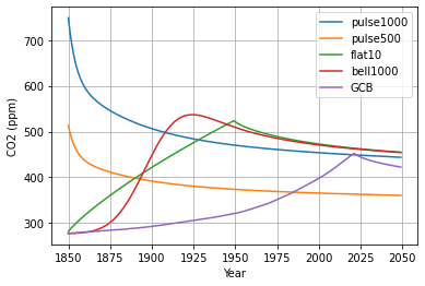
The solutions for the other idealized emissions profiles are plotted below.
The 1000 PgC cumulative emissions simulations all asymptote to the same eventual CO2 concentration of 381 ppm (104 ppm over preindustrial), since C0 = 0.22 * 1000 PgC/(2.12 PgC/ppm) = 104 ppm. The pulse1000 simulation is closer to this limit in 2050 since there’s been a longer time to exponentially decay within the 390 yr box. For the GCB simulation, C0 = 0.22 * 675 PgC/(2.12 PgC/ppm) = 70 ppm.
Also notable is that the GCB simulation hits a significantly larger CO2 maximum (452 ppm) than observed in 2022 (417 ppm). This is because the Impulse-Response formulation was tuned to 2010 conditions, when the airborne fraction was higher than earlier in the preindustrial period. This inaccuracy is a key reason the FaIR model uses a modification of this simple carbon cycle model.
FaIR Model Carbon Cycle (Millar et al 2017)
The fast impulse response model (FaIR) model has become a go-to tool for evaluating the impact of emissions on global temperature. It’s been used to determine whether a given emissions scenario falls under 1.5o C or 2o C of warming (e.g., Meinshausen et al 2022), for how much warming COVID-19 emissions reductions caused (Forster et al 2020), and the effect of airline emissions on climate (Klöwer et al 2021). The full parameterizations used in these analyses are discussed in Smith et al (2018) but the carbon cycle is described in Millar et al (2017), with further modifications made by Leach et al (2021).
Essentially FaIR uses the same Impulse-Response model described above (Joos et al 2013), with the addition of a variable timescale parameter α to represent the change in carbon uptake with climate state.
[latex]C(t)/P = a_0 + \sum_\limits{i=1}^{3}\ a_i\ e^{-t \over \alpha \tau_i}[/latex]
The equation above shows the time dependence of CO2 concentrations following a pulse of amplitude P.
With increases in temperature, and with increases in carbon dioxide taken up by the ocean and land, it becomes more difficult to take up additional CO2. The FaIR model lengthens the timescales of each box by a constant factor under these conditions. This parameterization targets a quantity called the integrated impulse response function (iIRF), which is the time-integrated fraction of carbon dioxide from an initial pulse that stays in the atmosphere over a specified time period. Here the integration time period is 100 years, so the quantity is called the iIRF100. Since the iIRF100 is integrated over time, it has units of years, and a value of iIRF100 = 50 years would indicate that on average over the 100 years time period, half of an emitted pulse of CO2 stays in the atmosphere.
The iIRF can be easily calculated with the concentration expression above:
[latex]iIRF_{100} = 100 a_0 + \sum_\limits{i=1}^3 \alpha a_i \tau_i (1 - exp({-100 \over \alpha \tau_i}))[/latex]
Then α is calculated by assuming that the iIRF100 is a linear function of temperature and of accumulated carbon in land and ocean sinks:
[latex]iIRF_{100} = r_0 + r_C C_{acc} + r_T T[/latex]
where Cacc = E – C is the accumulated carbon in land and ocean sinks. In Millar et al (2017), the parameters take these values: r0 = 32 yrs, rC = 19 yrs/Tt C, and rT = 4.2 yrs/K.
Leach et al. (2021) added rA, a proportionality parameter to the atmospheric CO2 increase, and renamed rC to ru, and made other notational changes (including changing indices).
[latex]iIRF_{100} = r_0 + r_u C_{acc} + r_T T + r_A C[/latex]
which means we can write in terms of E and C alone as
[latex]iIRF_{100} = r_0 + r_u E + r_T T + (r_A -r_u) C[/latex]
The alpha parameter can be solved by looking for roots of the equation
[latex]f(x) = \sum_\limits{i=1}^3 \alpha a_i \tau_i (1 - exp({-100 \over \alpha \tau_i})) + 100 a_0 - r_0 - r_C C_{acc} - r_T T[/latex]
This can be done iteratively with Newton’s method, noting that the alpha derivative of the above equation is
[latex]df/d\alpha = \sum_\limits{i=1}^3 a_i \tau_i (1 - exp({-100 \over \alpha \tau_i})) - 100 \alpha^{-1} a_i (exp({-100 \over \alpha \tau_i}))[/latex]
To avoid solving the nonlinear equation, Leach et al (2021) instead created a function based on the Newton’s method approximation:
[latex]\alpha = g_0 exp(g_1^{-1}(r_0 + r_u E + r_T T + (r_A - r_u) C))[/latex]
where the two g coefficients are only a function of the tau and a parameters, and thus do not change in perturbed parameter simulations.
[latex]g_1 = 100 a_0 + \sum_\limits{i=1}^3 a_i \tau_i (1 - (1+100/\tau_i) exp({-100 \over \tau_i}))=11.41262243 = (0.0876)^{-1}[/latex]
[latex]g_0 = exp(-g_1^{-1}(100 a_0 + \sum_\limits{i=1}^3 a_i \tau_i (1 - exp({-100 \over \tau_i})))) = 0.010178288[/latex]
Let’s examine the new direct solution for alpha from Leach et al (2021). Written in terms of a single leading coefficient
[latex]\alpha = \alpha_0 exp(\xi_E E + \xi_T T + \xi_{\kappa} C))[/latex]
with
[latex]\alpha_0 = g_0 exp(g_1^{-1} r_0)[/latex]
which takes values of α0 = 0.165 (0.10-0.40) for r0 = 32 (26.4-42.2) yr;
[latex]\xi_E = g_1^{-1} r_u[/latex]
which takes values of ξE = 0.26 (-0.53-1.05) yr/Tt for ru = 3 (-6-12) yr/Tt, and an amplification factor of 1.3 (0.59-2.86) for 1 Tt of cumulative emissions;
[latex]\xi_T = g_1^{-1} r_T[/latex]
which takes values of ξT = 0.2 (-0.25-0.71) yr/K for rT = 2.28 (-2.85-8.11) yr/K, and an amplification factor of 1.22 (0.78-2) for 1 K of warming;
and
[latex]\xi_{\kappa} = g_1^{-1} (r_A - r_u)[/latex]
which takes values of ξκ = -0.09 (-1.24-1.18) yr/Tt for rA-rU = -1.1 (-14.2-13.5) yr/Tt, and an amplification factor of 0.91 (0.29-3.26) for 1 Tt of atmospheric carbon increase (417 ppm CO2 increase). Note that cumulative emissions, temperature and atmospheric carbon each have a separable, multiplicative effect on the timescales.
Several unusual aspects of the Impulse-Response Model remain. For instance, although timescales now vary, the fraction of emissions that goes into each box (the ai parameters) stay fixed. So the amount of carbon that goes into the chemical weathering (τ = infinity) box is independent of temperature and accumulated carbon. Tuning the impulse-response model to preindustrial conditions in the Joos et al paper resulted in an a0 value that is nearly 30% smaller however, suggesting a fundamental mismatch at long timescales for this parameterization. For the 1850 to 2022 observed cumulative emissions EC = 675 PgC, the amount of atmospheric carbon in the chemical weathering box is C0 = 0.22 * 675 PgC/(2.12 PgC/ppm = 70 ppm, the same as the Joos et al (2013) model.
Parameters in FaIR can be varied in order to produce a probabilistic distribution of carbon states for each experiment. In the Dvorak et al (2022) study, we varied each of the three r parameters over wide prior distribution ranges, and then constrained the model by only considering the values that end up with CO2 concentrations close to today’s. Both rC and rT were essentially unconstrained from observations, so their distributions are the same as the prior distributions (set based on expectations from Earth system models, rT ~ 3-5 yrs/K and rC ~ 16-22 yrs/TtC). The atmospheric carbon dioxide partitioning for a “World Without Industry 2023” simulation is plotted below.
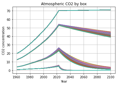
Note that most carbon is stored in box 0, the chemical weathering box, which experiences no decrease in concentration after emissions cease (there is actually a small increase, due to methane reacting into CO2 as CH4 concentration decreases exponentially). The value of 70 ppm means that CO2 concentrations are doomed to exceed 280 ppm + 70 ppm = 350 ppm for eternity in this model. The majority of the variance of atmospheric CO2 concentration after industry disappears is due to boxes 1 (deep ocean) and 2 (land).
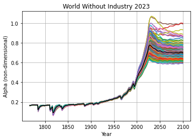
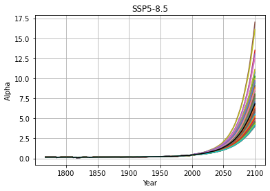
The alpha parameter varies by a large amount in both World Without Industry 2023 and SSP5-8.5:
 |
 |
Each simulation begins with α ≈ 0.2, meaning timescales are reduced by a factor of 5 initially, reflecting larger uptake into the atmosphere and the ocean in the preindustrial climate. Alpha exceeds 1 in only a few ensemble members in the WWI 2023 experiment, indicating that the timescales remain shorter than the Impulse-Response Model for nearly all times in this simulation. It should be noted that when alpha is small enough to make the smallest relaxation time on the order of 1 year (as in the preindustrial parameter set), there is a chance of numerical instability, so care should be taken when integrating these equations.
In the SSP5-8.5 experiment, α gets extremely large, experiencing an increase of nearly a factor of 100 in some ensemble members. The median has α = 7 by 2100, implying timescales of 2700 yrs, 260 yrs, and 30 yrs for boxes 1, 2 and 3. Note that over this entire range, the fraction of emissions that go into each box at a given time remains the same in all cases, so no matter the relaxation time, 22% of emissions still goes into the chemical weathering box, with no removal.
We can perform some simpler experiments with the FaIR carbon cycle, taking advantage of the fact that observed time series exist for E, T, and C. Let’s prescribe all of these (even C) and calculate the CO2 concentrations for various sets of parameters r0, ru, rT, and rA. For verification, we compare with the observed C time series.
Simple experiments with FaIR
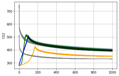
Let’s run the simple emissions experiments with FaIR, using 1000 members of the Dvorak et al (2022) ensemble tuned to the historical record. Our simulations are first spun-up for 1500 years using preindustrial (1850) conditions. Following the large spin-up, experiments are run for 1000 years. Carbon dioxide is plotted below.
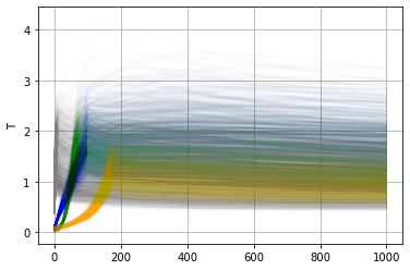
Gray curves are pulse1000 and pulse500 simulations, orange is GCB (historical), green is bell1000, and blue is flat10. Temperature is plotted below.
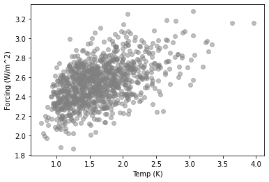
Obviously a lot of the spread in the above plot comes from the imposed range in climate sensitivity. How much does the forcing of CO2 change across these simulations? We plot CO2 forcing versus temperature across ensemble members for the pulse1000 experiment, 200 years after the pulse.
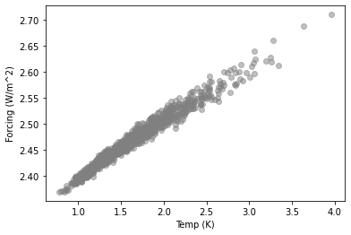
There’s a large range of CO2 forcing across the ensemble, from 1.8 to 3.3 W/m2. But one aspect of the ensemble scales CO2 forcing across ensemble members (with mean and standard deviation of the prior distribution set to match the IPCC forcing range as estimated in 2014). We can divide by this scaling to get an even better linear agreement between unscaled forcing and temperature.
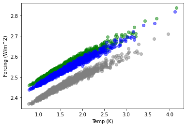
The regression slope in the above is 0.11 W/m2/K. If one compares the other two 1000 PgC simulations, similar slopes are calculated.
Gray is pulse1000, green is flat10, and blue is bell1000. All values are unscaled, i.e., the model CO2 forcing divided by the CO2 forcing scaling.
Let’s attempt to calculate the strength of the carbon cycle-temperature feedback, by calculating the change in CO2 concentration (and thus radiative forcing) from a small increase in temperature. The iIRF changes by 3-5 yr/K due to temperature change, depending on ensemble member. This causes about a 10% change in timescale. If we assume it’s mostly the 400 year box that affects concentrations in our selected year, then the concentration follows the equation
[latex]C = C_0 e^{- t / \alpha \tau}[/latex]
where C0 = 104 ppm, t = 200 years, tau = 400 yrs, and alpha, which satisfies the equation (to do: calculate the nonlinear solutions for alpha under these assumptions).
[latex]r_0 + r_C C' + r_T T = 100 a_0 + \alpha a_1 \tau_1 (1 - exp({-100 / \alpha \tau_1}))[/latex]
We solve
[latex]\alpha = (r_0 + r_C C' + r_T T - 100 a_0 ) (a_1 \tau_1 (1 - exp({-100 / \alpha \tau_1})))^{-1}[/latex]
Hector land carbon cycle (Hartin et al 2015)
Clearly the FaIR model is lacking in some of its parameterizations, so let’s explore physics-based models. Hector, first described in Hartin et al 2015, is a model with both active land and ocean.
Hector’s full carbon cycle is
[latex]{d C_{ATM} \over dt} = F_A + F_{LC} - F_O - F_L[/latex]
where CATM is the atmospheric carbon content, FA is the anthropogenic fossil fuel emissions, FLC is the land use change emissions, FO is the ocean carbon uptake, and FL is the land carbon uptake. We’ll explore the land parameterization first, to calculate FL.
Land carbon uptake consists of sources and sinks, with FL = NPP – RH, with NPP the net primary production (photosynthesis taking up CO2) and RH is heterotrophic respiration (microbes breaking down soils and releasing CO2). These change with both temperature (microbial activity accelerating in warmer climates) and ambient CO2 concentration (photosynthesis increasing with more CO2 in the air). For parameterizations of these, we need to consider reservoirs of carbon on land, in vegetation (CV), detritus (CD, mostly fallen leaves), and soil (CS), and equations for these add quite a few parameters:
[latex]{dC_V \over dt} = f_{nv} NPP - (f_{vd} + f_{vs}) C_V - f_{lv} F_{LC}[/latex]
[latex]{dC_D \over dt} = f_{nd} NPP + f_{vd} C_V - f_{ds} C_D - RH_D - f_{ld} F_{LC}[/latex]
[latex]{dC_S \over dt} = f_{ns} NPP + f_{vs} C_V + f_{ds} C_D - RH_S - f_{ls} F_{LC}[/latex]
Let’s examine the sum of these first in order to better understand the overall behavior of the system. Noting that [latex]f_{nv} + f_{nd} + f_{ns} = f_{lv} + f_{ld} + f_{ls} = 1[/latex],
[latex]{d(C_V + C_D + C_S) \over dt} = NPP - F_{LC} - RH[/latex]
where RH = RHD + RHS. Adding to this to the full carbon cycle equation above gives
[latex]{d(C_V + C_D + C_S + C_{ATM}) \over dt} = F_{A} - F_{O}[/latex].
Consider interactions between the land and atmosphere only (FO = 0). The above equation shows that any nonzero anthropogenic emissions source (from fossil fuels, i.e., FA) cannot be balanced by changes in the land. Fossil fuel emissions must go to zero to reach any kind of equilibrium, no matter what functional forms are chosen for NPP and RH. Land use change, on the other hand, can be supported in equilibrium, if FLC = FL., i.e., if NPP – RH = FLC.
With the overall conservation law in mind, let’s consider the parameterizations of NPP and RH in Hector.
[latex]NPP = NPP_0 (1 + \beta log(C_{ATM}/C_0))[/latex]
[latex]RH_D = C_D f_{rd}*Q_{10}^{T/10}[/latex]
[latex]RH_S = C_S f_{rs}*Q_{10}^{T/10}[/latex]
The temperature in the heterotrophic respiration functions is sometimes taken to be an average over several previous years (10 years for this version of the model). Parameter values for the land equations are given below.
| Vegetation | Detritus | Soil | |
| NPP partitioning | fnv = 0.35 | fnd = 0.6 | fns = 0.05 |
| Land use partitioning | flv = 0.1 | fld = 0.01 | fls = 0.89 |
| Fluxes from (to) | fvd = 0.034 yr-1 (to detritus) | fds = 0.6 yr-1 (to soil) | |
| fvs = 0.001 yr-1 (to soil) | |||
| Respiration coefficients | frd = 0.25 yr-1 | frs = 0.02 yr-1 | |
| Preindustrial reservoir size | 550 PgC | 55 PgC | 1782 PgC |
Other parameter values are β = 0.36, Q10 = 2.45, NPP0 = 50 PgC/yr, and preindustrial atmospheric carbon CA0 = 588 PgC (equivalent to 277 ppm). A spinup simulation is necessary to take the preindustrial initial conditions to an equilibrium (which is similar to the parameters listed above). Then experiments are run relative to the equilibrated preindustrial state.
Let’s analyze the equations to gain some intuition about their behavior, first with the vegetation equation. In steady state, with no land use emissions,
[latex]C_V = {f_{nv} \over f_{vd} + f_{vs}}\\ \ \ \ \ \ = 10\ NPP[/latex]
This relation relaxes with a timescale of (fvd + fvs)-1 = 28.6 years.
The relaxation time of the detritus equation is much shorter, (fds + frd Q10T/10)-1 = (0.6 + 0.25 Q10T/10)-1, equivalent to only 1.2 years when the temperature change is small. This may cause numerical difficulties since the timestep is only 1 year. One might consider implementing an equilibrated detritus equation for numerical stability:
[latex]C_D = (f_{ns}\ NPP + f_{vs} C_V ) / (f_{ds} + f_{rd}\ Q_{10}^{T/10})\\ \ \ \ \ \ = (0.6\ NPP + 0.034\ C_V)/(0.6\ + 0.25\ Q_{10}^{T/10})[/latex]
In equilibrium, with small temperature change, CD = 1.1 NPP.
Finally, the soil equation has a relaxation time of 1/frs = 50 years, and has an equilibrium value of CS = 36 NPP with small temperature change.
[latex]C_S = f_{rs}^{-1} [(f_{ns} + f_{nv})\ NPP\ Q_{10}^{-T/10} - f_{rd}\ C_D][/latex]
Next let’s consider the response to a pulse of emissions with amplitude P, applied to the land and atmosphere in an equilibrated preindustrial basic state. We’ll refer to perturbation from the equilibrated state with primes. Conservation of carbon requires that
[latex]C_A' + C_V' + C_D' + C_S' = P[/latex]
The pulse starts in the atmosphere, and is first distributed into the land by increases in NPP, in response to higher CO2 levels. Anomalous NPP takes the form
[latex]NPP' = \beta \ NPP_0\ log(1 + C_A' / C_{A0})[/latex]
with preindustrial atmospheric carbon CA0 = 277 ppm. For small changes in atmospheric CO2,
[latex]NPP' = \beta \ NPP_0\ C_A' / C_{A0}[/latex]
β NPP0 / CA0 has units of inverse timescale and is equal to (0.36) (50 PgC/yr) / (588 PgC) = 1/32.7 years.
To add… some plots of response of land reservoirs and CO2 to pulses of emissions.
Ocean Carbon Cycle in BEAM (Glotter et al 2014)
The Bolin and Erikkson Adjusted Model (BEAM) was developed as a simple carbon cycle that could be used in place of a highly erroneous carbon cycle model used in the (Nobel Memorial Prize-winning) Dynamic Integrated model of Climate and the Environment (DICE) model of Nordhaus. DICE gives errors of up to 2o C at 2300 and 6o C in 3500 compared with comprehensive models. BEAM consists of three boxes, for the atmosphere, upper ocean and lower ocean.
[latex]{dM_{at} \over dt} = E(t) - k_a (M_{at} - A\ B M_{up})[/latex]
[latex]{dM_{up} \over dt} =k_a (M_{at} - A\ B M_{up}) - k_d (M_{up} - M_{lo}/\delta)[/latex]
[latex]{dM_{lo} \over dt} = k_d (M_{up} - M_{lo}/\delta)[/latex]
where Mat, Mup, and Mlo are the mass of inorganic carbon of the atmosphere, upper ocean and lower ocean, respectively; ka and kd are inverse exchange timescales for the atmosphere-upper ocean and upper-lower ocean; δ is the ratio between volumes of lower and upper ocean (~50), and A B is the equilibrium ratio of atmosphere to upper ocean inorganic carbon. It’s separated into the product of two terms, A, the ratio between atmosphere and ocean CO2 concentration at equilibrium (a function of temperature, since a warmer ocean holds less CO2), and B, the ratio between dissolved CO2 to inorganic carbon at equilibrium (a strong function of pH, with a more acidic ocean holding much less inorganic carbon).
In this model, Mat – A B Mup is the disequilibrium between atmospheric and upper ocean inorganic carbon, eroded with rate 1/ka, and Mup – Mlo/δ is the disequilibrium between upper and lower ocean inorganic carbon, eroded with rate 1/kd. Uptake occurs whenever Mat > A B Mup and A B increases substantially with increased acidity. In order to parameterize these terms we need to do some chemistry.
CO2 + H2O ↔ HCO3 + H+ ↔ CO3 + 2 H+
Dissolved CO2 (carbonic acid) partitions with bicarbonate and with carbonate instantaneously. Ratios between these is set by partitioning coefficients k1 (to dissociate once) and k2 (to dissociate a second time), and concentration of H+ ions (i.e., pH = -log10 H+).
A = kH AM/(OM/(δ+1))
B-1 = 1 + k1/H+ + k1 k2/H+2
Etc
FaIR has the same partitioning but different relaxation times, due in part to the carbon uptake and in part due to the temperature change. The latter requires the use of a climate model, and an expression for radiative forcing from CO2 concentrations. Each of these add uncertainty in any estimate of future CO2 levels. We can bracket the changes in carbon cycle by examining the iIRF100 expression parameterization:
[latex]iIRF_{100} = r_0 + r_C C_{acc} + r_T T[/latex]
with median values of r0 = 32 yrs, rC = 19 yrs/Tt and rT = 4.2 yrs/K. With a total emissions of 0.1 TtC, the eventual change from carbon uptake is 0.78 * 1.9 yrs = 1.5 yrs, around 5%. With a temperature change of 0.35 K (near the high end of warming estimated by simple climate models for this experiment), the temperature-induced change in iIRF100 is also 1.5 yrs. In total, this means relaxation times will be lengthened by around 10% due to the climate and carbon uptake changes in this scenario. Recall however that the FaIR model starts with a different set of relaxation times in preindustrial, with alpha = 0.2. So the FaIR simulations will have much shorter relaxation times throughout this simulation, and should accumulate much less carbon in the atmosphere from the pulse emissions.
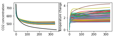
While the Impulse-Response model has no amplitude dependence, FaIR’s response depends on both the total carbon taken up and the temperature change. Consider instead a 1 TtC pulse (equivalent to the total emissions of the flat10 experiment, applied all at once). For this, the eventual carbon uptake of 0.78 TtC will cause a change in iIRF100 of 15 yrs, and temperature changes might cause an additional 8-24 yr change in iIRF100. This can double the initial iIRF100 value of 32 yrs, and extend the relaxation times to a larger value than the Impulse-Response model. So one might expect an initial faster decrease of CO2 levels in FaIR in the experiment, quickly followed by slower relaxation times and higher CO2 levels for several hundred years. Results from a 1 TtC pulse experiment are shown below, with the Impulse-Response solution in black, and the FaIR calibrated ensemble in colors.
Let’s next consider the flat10 experiment.

